Statistical Performance Comparisons of Computers Tianshi Chen 1 , - PowerPoint PPT Presentation
Statistical Performance Comparisons of Computers Tianshi Chen 1 , Yunji Chen 1 , Qi Guo 1 , Olivier Temam 2 , Yue Wu 1 , Weiwu Hu 1 1 State Key Laboratory of Computer Architecture, Institute of Computing Technology (ICT), Chinese Academy of
Statistical Performance Comparisons of Computers Tianshi Chen 1 , Yunji Chen 1 , Qi Guo 1 , Olivier Temam 2 , Yue Wu 1 , Weiwu Hu 1 1 State Key Laboratory of Computer Architecture, Institute of Computing Technology (ICT), Chinese Academy of Sciences, Beijing, China 2 National Institute for Research in Computer Science and Control (INRIA), Saclay, France HPCA-18, New Orleans, Louisiana Feb. 28th, 2012
Outline Motivation Empirical Observations Our Proposal Outline 1 Motivation 2 Empirical Observations 3 Our Proposal Chen et al. Statistical Performance Comparisons of Computers
Outline Motivation Empirical Observations Our Proposal Performance comparisons of computers: the tradition We need. . . A number of benchmarks (e.g., SPEC CPU2006, SPLASH-2) Basic performance metrics (e.g., IPC, delay) Single-number performance measure (e.g., geometric mean; “War of means” [Mashey, 2004] The danger Performance variability of computers Example 10 subsequent runs of SPLASH-2 on a commodity computer Geometric mean performance speedups, over an initial baseline run are 0.94, 0.98, 1.03, 0.99, 1.02, 1.03, 0.99, 1.10, 0.98, 1.01 Deterministic trend vs. Stochastic fluctuation We need to estimate the confidence/reliability of each comparison result! Chen et al. Statistical Performance Comparisons of Computers
Outline Motivation Empirical Observations Our Proposal An example Quantitative performance comparison: estimating the performance speedup of computer “PowerEdge T710” over “Xserve” (using SPEC CPU2006 data collected from SPEC.org) Speedup obtained by comparing their geometric mean SPEC ratios: 3 . 50 Confidence of the above speedup, obtained by our proposal: 0.31 ( If we don’t estimate the confidence, we would not know that the comparison result is rather dangerous ) Speedup obtained by our proposal: 2 . 23 (with the confidence 0.95) Chen et al. Statistical Performance Comparisons of Computers
Outline Motivation Empirical Observations Our Proposal Performance comparisons of computers: the tradition Traditional solutions: basic parametric statistical techniques Confidence Interval t -test [Student (W. S. Gosset), 1908] Preconditions Performance measurements should be normally-distributed Otherwise, number of performance measurements must be large enough [Le Cam, 1986] Lindeberg-L´ evy Central Limit Theorem : let { x 1 , x 2 , . . . , x n } be a size- n sample consisting of n measurements of the same non-normal distribution with mean 휇 and finite variance 휎 2 , and S n = ( ∑ n i =1 x i ) / n be the mean of the measurements (i.e., sample mean). When n → ∞ , √ n ( S n − 휇 ) d → 풩 (0 , 휎 2 ) − (1) Our practices : 20–30 benchmarks (e.g., SPEC CPU2006), each is run for 3 (or fewer) times Chen et al. Statistical Performance Comparisons of Computers
Outline Motivation Empirical Observations Our Proposal Another example Consider ratios of two commodity computers A (upper) and B (lower) on SPECint2006 (collected from SPEC.org) Intuitive observation: A beats B on all 12 benchmarks Paired t -test: at the confidence level ≥ 0 . 95, A does not significantly outperform B ! Reason: t -statistic is constructed by the sample mean and the variance . Chen et al. Statistical Performance Comparisons of Computers
Outline Motivation Empirical Observations Our Proposal Another example Why? t -statistic is constructed by the sample mean and the variance. The shape of a non-normal and skewed distribution will be stretched if we consider it to be normal. The performance score of A is incorrectly considered to obey the normal distribution 풩 (79 . 63 , 174 . 67 2 ) (79 . 63 ± 174 . 67). In other words, the performance score of A takes a large probability to be negative ! But in fact, the performance scores of A are in the interval (20 , 634). Chen et al. Statistical Performance Comparisons of Computers
Outline Motivation Empirical Observations Our Proposal Another example Consider ratios of two commodity computers A (upper) and B (lower) on SPECint2006 (collected from SPEC.org) Paired t -test: at the confidence level ≥ 0 . 95, A does not significantly outperform B ! In practice, parametric techniques are quite vulnerable to performance outliers which apparently break the normality Performance outliers are common (e.g., specialized architecture performing very well on specific applications)! Chen et al. Statistical Performance Comparisons of Computers
Outline Motivation Empirical Observations Our Proposal Outline 1 Motivation 2 Empirical Observations 3 Our Proposal Chen et al. Statistical Performance Comparisons of Computers
Outline Motivation Empirical Observations Our Proposal Settings Commodity computers Intel i7 920 (4-core 8-thread), 6 GB DDR2 RAM, Linux OS Intel Xeon dualcore, 2GB RAM, Linux OS Benchmarks SPEC CPU2000 & CPU2006 SPLASH-2, PARSEC KDataSets (MiBench) [Guthaus et al., 2001; Chen et al., 2010] Online repository of SPEC.org Chen et al. Statistical Performance Comparisons of Computers
Outline Motivation Empirical Observations Our Proposal We need to study. . . Do performance measurements distribute normally? If not, whether the common number of performance measurements is large enough (for making the Central Limit Theorem applicable)? If we get two “No” above, how to carry out performance comparisons? Chen et al. Statistical Performance Comparisons of Computers
Outline Motivation Empirical Observations Our Proposal Do performance measurements distribute normally? Naive Normality Fitting (NNF) assumes that the execution time distributes normally, and estimates the normal distribution Kernel Parzen Window (KPW) [Parzen, 1962] directly estimates the real distribution of execution time If KPW-curve ∕ =NNF-curve, then the execution time does not obey a normal law −3 Equake, SPEC CPU2000 (10000 Runs) −4 Raytrace, SPLASH−2 (10000 Runs) −4 Swaptions, PARSEC (10000 Runs) x 10 x 10 x 10 1.4 1.6 1.2 1.4 1.2 Sample Mean Sample Mean Sample Mean 1 1.2 Probability Density Probability Density 1 Probability Density 0.8 1 0.8 0.8 0.6 0.6 0.6 0.4 0.4 0.4 0.2 0.2 0.2 0 0 0 2.18 2.2 2.22 2.24 2.26 2.28 2.3 5.41 5.61 5.81 6.01 6.21 6.41 6.61 6.8 6.3 6.8 7.3 7.8 8.3 8.6 Execution Time (us) 5 Execution Time (us) 5 Execution Time (us) 5 x 10 x 10 x 10 Chen et al. Statistical Performance Comparisons of Computers
Outline Motivation Empirical Observations Our Proposal Do performance measurements distribute normally? −3 Equake, SPEC CPU2000 (10000 Runs) −4 Raytrace, SPLASH−2 (10000 Runs) −4 Swaptions, PARSEC (10000 Runs) x 10 x 10 x 10 1.4 1.6 1.2 1.4 1.2 Sample Mean Sample Mean Sample Mean 1 1.2 Probability Density Probability Density 1 Probability Density 1 0.8 0.8 0.8 0.6 0.6 0.6 0.4 0.4 0.4 0.2 0.2 0.2 0 0 0 2.18 2.2 2.22 2.24 2.26 2.28 2.3 5.41 5.61 5.81 6.01 6.21 6.41 6.61 6.8 6.3 6.8 7.3 7.8 8.3 8.6 Execution Time (us) Execution Time (us) Execution Time (us) 5 5 5 x 10 x 10 x 10 Long tails, especially for multi-threaded benchmarks. The distributions of the execution times on Raytrace and Swaptions seem to be power-law . It’s hard for a program (especially multi-threaded ones) to execute faster than a threshold, but easy to be slowed down by, for example, data races, thread scheduling, synchronization order, and contentions of shared resources. Chen et al. Statistical Performance Comparisons of Computers
Outline Motivation Empirical Observations Our Proposal Do performance measurements distribute normally? Do cross-benchmark performance measurements distribute normally? CPU2006 data of 20 computers collected from from SPEC.org Statistical normality test At the confidence level of 0.95, the answer is significantly “No” to all 20 computers over SPEC CPU2006, 19 out of 20 over SPECint2006, 18 out of 20 over SPECfp2006 Chen et al. Statistical Performance Comparisons of Computers
Outline Motivation Empirical Observations Our Proposal Whether the Central Limit Theorem (CLT) is applicable? Briefly, the CLT states that the mean of a sample (with a number of measurements) distributes normally when the sample size (number of measurements in the sample) is sufficiently-large . How large is “sufficiently-large”? Empirical study on performance data w.r.t. KDataSets 32,000 different combinations of benchmarks and data sets (thus 32,000 IPC scores) are available Randomly collect 150 samples from the 32,000 scores, each consists of n randomly selected scores 150 observations of the sample mean have been enough for exhibiting the normality (if the normality holds) The sample size n is set to 10, 20, 40, 60, . . . , 240, 260, 280 in 15 different trials, respectively Chen et al. Statistical Performance Comparisons of Computers
Recommend
More recommend
Explore More Topics
Stay informed with curated content and fresh updates.
