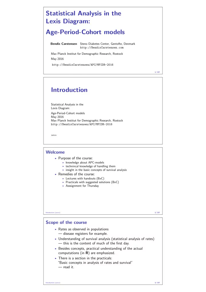

Statistical Analysis in the Lexis Diagram: Age-Period-Cohort models Bendix Carstensen Steno Diabetes Center, Gentofte, Denmark http://BendixCarstensen.com Max Planck Institut for Demographic Research, Rostock May 2016 http://BendixCarstensen/APC/MPIDR-2016 1/ 327 Introduction Statistical Analysis in the Lexis Diagram: Age-Period-Cohort models May 2016 Max Planck Institut for Demographic Research, Rostock http://BendixCarstensen/APC/MPIDR-2016 intro Welcome ◮ Purpose of the course: ◮ knowledge about APC-models ◮ technincal knowledge of handling them ◮ insight in the basic concepts of survival analysis ◮ Remedies of the course: ◮ Lectures with handouts (BxC) ◮ Practicals with suggested solutions (BxC) ◮ Asssignment for Thursday Introduction ( intro ) 2/ 327 Scope of the course ◮ Rates as observed in populations — disease registers for example. ◮ Understanding of survival analysis (statistical analysis of rates) — this is the content of much of the first day. ◮ Besides concepts, practical understanding of the actual computations (in R ) are emphasized. ◮ There is a section in the practicals: “Basic concepts in analysis of rates and survival” — read it. Introduction ( intro ) 3/ 327
About the lectures ◮ Please interrupt: Most likely I did a mistake or left out a crucial argument. ◮ The handouts are not perfect — please comment on them, prospective students would benefit from it. ◮ There is a time-schedule in the practicals. It might need revision as we go. Introduction ( intro ) 4/ 327 About the practicals ◮ You should use you preferred R -enviroment. ◮ Epi -package for R is needed. ◮ Data are all on my website. ◮ Try to make a text version of the answers to the exercises — it is more rewarding than just looking at output. The latter is soon forgotten. ◮ An opportunity to learn emacs , ESS and Sweave ? Introduction ( intro ) 5/ 327 Rates and Survival Statistical Analysis in the Lexis Diagram: Age-Period-Cohort models May 2016 Max Planck Institut for Demographic Research, Rostock http://BendixCarstensen/APC/MPIDR-2016 surv-rate Survival data ◮ Persons enter the study at some date. ◮ Persons exit at a later date, either dead or alive. ◮ Observation: ◮ Actual time span to death ( “event” ) ◮ . . . or . . . ◮ Some time alive ( “at least this long” ) Rates and Survival ( surv-rate ) 6/ 327
Examples of time-to-event measurements ◮ Time from diagnosis of cancer to death. ◮ Time from randomisation to death in a cancer clinical trial ◮ Time from HIV infection to AIDS. ◮ Time from marriage to 1st child birth. ◮ Time from marriage to divorce. ◮ Time from jail release to re-offending Rates and Survival ( surv-rate ) 7/ 327 ● Each line a person ● ● ● ● ● ● Each blob a death ● ● ● ● Study ended at 31 ● Dec. 2003 ● ● ● ● ● ● ● ● ● ● ● ● ● ● ● ● 1993 1995 1997 1999 2001 2003 Calendar time Rates and Survival ( surv-rate ) 8/ 327 Ordered by date of ● ● entry ● ● Most likely the ● order in your ● ● database. ● ● ● ● ● ● ● ● ● ● ● ● ● ● ● ● ● ● ● ● ● 1993 1995 1997 1999 2001 2003 Calendar time Rates and Survival ( surv-rate ) 9/ 327 Timescale changed ● ● to ● “Time since ● diagnosis” . ● ● ● ● ● ● ● ● ● ● ● ● ● ● ● ● ● ● ● ● ● ● ● ● 0 2 4 6 8 10 Time since diagnosis Rates and Survival ( surv-rate ) 10/ 327
● ● Patients ordered by ● ● ● ● ● ● survival time. ● ● ● ● ● ● ● ● ● ● ● ● ● ● ● ● ● ● ● ● 0 2 4 6 8 10 Time since diagnosis Rates and Survival ( surv-rate ) 11/ 327 ● ● Survival times ● ● ● ● ● ● grouped into bands ● ● ● ● ● of survival. ● ● ● ● ● ● ● ● ● ● ● ● ● ● ● 1 2 3 4 5 6 7 8 9 10 Year of follow−up Rates and Survival ( surv-rate ) 12/ 327 ● ● ● ● ● Patients ordered by ● ● ● ● ● ● ● survival status ● ● ● within each band. ● ● ● ● ● ● ● ● ● ● ● ● ● 1 2 3 4 5 6 7 8 9 10 Year of follow−up Rates and Survival ( surv-rate ) 13/ 327 Survival after Cervix cancer Stage I Stage II Year N D L N D L 1 110 5 5 234 24 3 2 100 7 7 207 27 11 3 86 7 7 169 31 9 4 72 3 8 129 17 7 5 61 0 7 105 7 13 6 54 2 10 85 6 6 7 42 3 6 73 5 6 8 33 0 5 62 3 10 9 28 0 4 49 2 13 10 24 1 8 34 4 6 Estimated risk in year 1 for Stage I women is 5 / 107 . 5 = 0 . 0465 Estimated 1 year survival is 1 − 0 . 0465 = 0 . 9535 — Life-table estimator. Rates and Survival ( surv-rate ) 14/ 327
Survival function Persons enter at time 0 : Date of birth Date of randomization Date of diagnosis. How long they survive, survival time T — a stochastic variable. Distribution is characterized by the survival function: S ( t ) = P { survival at least till t } = P { T > t } = 1 − P { T ≤ t } = 1 − F ( t ) Rates and Survival ( surv-rate ) 15/ 327 Intensity or rate λ ( t ) = P { event in ( t , t + h ] | alive at t } / h = F ( t + h ) − F ( t ) S ( t ) × h = − S ( t + h ) − S ( t ) h → 0 − dlog S ( t ) − → S ( t ) h d t This is the intensity or hazard function for the distribution. Characterizes the survival distribution as does f or F . Theoretical counterpart of a rate . Rates and Survival ( surv-rate ) 16/ 327 Relationships − dlog S ( t ) = λ ( t ) d t � � t � � S ( t ) = exp − λ ( u ) d u = exp ( − Λ( t )) 0 � t Λ( t ) = 0 λ ( s ) d s is called the integrated intensity or cumulative hazard . Λ( t ) is not an intensity — it is dimensionless. Rates and Survival ( surv-rate ) 17/ 327 Rate and survival � t � � λ ( t ) = − S ′ ( t ) S ( t ) = exp − λ ( s ) d s S ( t ) 0 ◮ Survival is a cumulative measure ◮ A rate is an instantaneous measure. ◮ Note: A cumulative measure requires an origin! Rates and Survival ( surv-rate ) 18/ 327
Observed survival and rate ◮ Survival studies: Observation of (right censored) survival time: δ = 1 { X = T } X = min( T , Z ) , — sometimes conditional on T > t 0 , (left truncated). ◮ Epidemiological studies: Observation of (components of) a rate: D , Y , D / Y D : no. events, Y no of person-years. Rates and Survival ( surv-rate ) 19/ 327 Empirical rates for individuals ◮ At the individual level we introduce the empirical rate: ( d , y ) , — no. of events ( d ∈ { 0 , 1 } ) during y risk time ◮ Each person may contribute several empirical ( d , y ) ◮ Empirical rates are responses in survival analysis ◮ The timescale is a covariate : — varies across empirical rates from one individual: Age, calendar time, time since diagnosis ◮ Do not confuse timescale with y — risk time (exposure in demograpy) a difference between two points on any timescale Rates and Survival ( surv-rate ) 20/ 327 Empirical rates by ● ● calendar time. ● ● ● ● ● ● ● ● ● ● ● ● ● ● ● ● ● ● ● ● ● ● ● ● ● ● 1993 1995 1997 1999 2001 2003 Calendar time Rates and Survival ( surv-rate ) 21/ 327 Empirical rates by ● ● time since diagnosis. ● ● ● ● ● ● ● ● ● ● ● ● ● ● ● ● ● ● ● ● ● ● ● ● ● ● 0 2 4 6 8 10 Time since diagnosis Rates and Survival ( surv-rate ) 22/ 327
Two timescales Note that we actually have two timescales: ◮ Time since diagnosis ( i.e. since entry into the study) ◮ Calendar time. These can be shown simultaneously in a Lexis diagram. Rates and Survival ( surv-rate ) 23/ 327 12 Follow-up by 10 calendar time ● and time since 8 Time since diagnosis diagnosis: ● ● 6 ● A Lexis ● ● diagram! 4 ● ● ● ● ● ● ● ● ● ● 2 ● ● ● ● ● ● ● ● ● ● ● ● 0 1994 1996 1998 2000 2002 2004 Rates and Survival ( surv-rate ) 24/ 327 Calendar time 12 Empirical rates 10 by ● calendar time and 8 Time since diagnosis time since ● ● diagnosis 6 ● ● ● 4 ● ● ● ● ● ● ● ● ● ● 2 ● ● ● ● ● ● ● ● ● ● ● ● 0 1994 1996 1998 2000 2002 2004 Rates and Survival ( surv-rate ) 25/ 327 Calendar time Likelihood for rates Statistical Analysis in the Lexis Diagram: Age-Period-Cohort models May 2016 Max Planck Institut for Demographic Research, Rostock http://BendixCarstensen/APC/MPIDR-2016 likelihood
Recommend
More recommend