Static analysis and all that Martin Steffen IfI UiO Spring 2014 - PowerPoint PPT Presentation

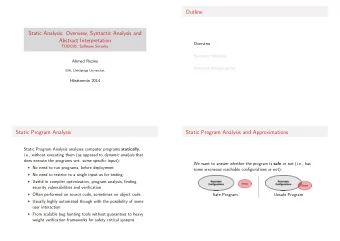
Static analysis and all that Martin Steffen IfI UiO Spring 2014 uio

Static analysis and all that Martin Steffen IfI UiO Spring 2014 uio

Plan • approx. 15 lectures, details see web-page • flexible time-schedule, depending on progress/interest • covering parts/following the structure of textbook [2], concentrating on • overview • data-flow • control-flow • type- and effect systems • helpful prior knowledge: having at least heard of • typed lambda calculi (especially for CFA) • simple type systems • operational semantics • lattice theory, fixpoints, induction

Introduction 1 Setting the scene Data-flow analysis Equational approach Constraint-based approach Constraint-based analysis Type and effect systems Algorithms

Plan • introduction/motivation into the field • short survey about the material: 5 main topics • data flow analysis • control flow analysis/constraint based analysis • [Abstract interpretation] • type and effect systems • [algorithmic issues] • 2 lessons

SA: why and what? • static: at “compile time” What: • analysis: deduction of program properties • automatic/decidable • formally, based on semantics • error catching Why: • enhancing program quality • catching common “stupid” errors without bothering the user much • spotting errors early • certain similarities to model checking • examples: type checking, uninitialized variables (potential nil-pointer deref’s), unused code • optimization: based on analysis, transform the “code” 1 , such the the result is “better” • examples: precalculation of results, optimized register allocation . . . success-story for formal methods 1 source code, intermediate code at various levels

Nature of SA • programs have differerent “semantical phases” • corresponding to Chomsky’s hierarchy • “static” = in principle: before run-time, but in praxis, “ context-free ” 2 • since: run-time most often: undecidable ⇒ static analysis as approximation • See [2, Figure 1.1] L0 L1 L2 L3 lexer parser sa exec. compile time run time 2 playing with words, one could call full-scale (hand?) verification “static” analysis, and likewise call lexical analysis a static analysis.

Phases machine indep. machine dep. optimizations optimizations code lexical syntactic stat. semantic analysis analysis checking generation symbol table stream of stream of machine syntax tree tokens syntax tree code char’s

SA as approximation universe unsafe exact safe over-approximation

While-language • simple, prototypical imperative language: • “untyped” • simple control structure: while, conditional, sequencing • simple data (numerals, booleans) • abstract syntax � = concrete syntax • disambiguation when needed: ( . . . ) , or { . . . } or begin . . . end a ::= x | n | a op a a arithm. expressions ::= true | false | not b | b op b b | a op r a b boolean expr. S ::= x := a | skip | S 1 ; S 2 statements if b then S else S | while b do S Table: Abstract syntax

While-language: labelling • associate flow information ⇒ labels • elementary block = labelled item • identify basic building blocks • unique labelling a ::= x | n | a op a a arithm. expressions b ::= true | false | not b | b op b b | a op r a boolean expr. [ x := a ] l | [ skip ] l | S 1 ; S 2 S ::= statements if [ b ] l then S else S | while [ b ] l do S Table: Abstract syntax

Example: factorial y := x ; z := 1 ; while y > 1 do ( z := z ∗ y ; y := y − 1 ); y := 0 • input variable: x • output variable: z

Example: factorial [ y := x ] 1 ; [ z := 1 ] 2 ; while [ y > 1 ] 3 do ([ z := z ∗ y ] 4 ; [ y := y − 1 ] 5 ); [ y := 0 ] 6 [ y := x ] 1 [ z := 1 ] 2 no [ y > 1 ] 3 [ y := 0 ] 6 yes [ z := z ∗ y ] 4 [ y := y − 1 ] 5

Reaching definitions analysis • “definition” of x : assignment to x : x := a • better name: reaching assignment analysis • first, simple example of data flow analysis assignment (= “definition”) [ x := a ] l may reach a pro- gram point, if there exists an execution where x was last assigned at l , when the mentioned program point is reached.

Factorial: reaching assignment [ y := x ] 1 [ z := 1 ] 2 no [ y > 1 ] 3 [ y := 0 ] 6 yes [ z := z ∗ y ] 4 [ y := y − 1 ] 5 • ( y , 1 ) (short for [ y := x ] 1 ) may reach: • the entry to 4 (short for [ z := z ∗ y ] 4 ). • the exit to 4 (not in the picture as arrow) • the entry to 5 • but: not the exit to 5

Factorial: reaching assignments • “points” in the program: entry and exit to elementary blocks/labels • ? : special label (not occurring otherwise), representing entry to the program, i.e., ( x , ?) represents initial (uninitialized) value of x • full information: pair of functions of type RD = ( RD entry , RD exit ) (1) l RD entry RD exit 1 ( x , ?) , ( y , ?) , ( z , ?) ( x , ?) , ( y , 1 ) , ( z , ?) 2 ( x , ?) , ( y , 1 ) , ( z , ?) ( x , ?) , ( y , 1 ) , ( z , 2 ) 3 ( x , ?) , ( y , 1 ) , ( y , 5 ) , ( z , 2 ) , ( z , 4 ) ( x , ?) , ( y , 1 ) , ( y , 5 ) , ( z , 2 ) , ( z , 4 ) 4 ( x , ?) , ( y , 1 ) , ( y , 5 ) , ( z , 2 ) , ( z , 4 ) ( x , ?) , ( y , 1 ) , ( y , 5 ) , ( z , 4 ) 5 ( x , ?) , ( y , 1 ) , ( y , 5 ) , ( z , 4 ) ( x , ?) , ( y , 5 ) , ( z , 4 ) 6 ( x , ?) , ( y , 1 ) , ( y , 5 ) , ( z , 2 ) , ( z , 4 ) ( x , ?) , ( y , 6 ) , ( z , 2 ) , ( z , 4 )

Reaching assignments: remarks • elementary blocks of the form • [ b ] l : entry/exit information coincides • [ x := a ] l : entry/exit information (in general) different • at program exit: ( x , ?) , x is input variable • table: “best” information = “smallest”: • additional pairs in the table: still safe • removing labels: unsafe • note: still an approximation • no real (= run time) data, no real execution, only data flow • approximate since • in concrete runs: at each point in that run, there is exactly one last assignment, not a set • label represents (potentially infinitely many) runs • e.g.: at program exit in concrete run: either ( z , 2 ) or else ( z , 4 )

Data flow analysis • standard: representation of program as flow graph • nodes: elementary blocks with labels • edges: flow of control • two approaches (both here quite similar) • equational approach • constraint-based approach

From flow graphs to equations • associate an equation system with the flow graph: • describing the “flow of information” • here: • the information related to reaching assignments • information imagined to flow forwards • solution of the equations • describe safe approximations • not unique, interest in the least (or largest ) solution • here: • give back RD of equation (1) on slide 16

Equations for RD and factorial: intra-block first type: local, “intra-block”: • flow through each individual block • relating for each elementary block its exit with its entry elementary block: [ y := x ] 1 RD exit ( 1 ) = RD entry ( 1 ) \{ ( y , l ) | l ∈ Lab } ∪ { ( y , 1 ) } (2)

Equations for RD and factorial: intra-block first type: local, “intra-block”: • flow through each individual block • relating for each elementary block its exit with its entry elementary block: [ y > 1 ] 3 RD exit ( 1 ) = RD entry ( 1 ) \{ ( y , l ) | l ∈ Lab } ∪ { ( y , 1 ) } (2) RD exit ( 3 ) = RD entry ( 3 )

Equations for RD and factorial: intra-block first type: local, “intra-block”: • flow through each individual block • relating for each elementary block its exit with its entry all equations with RD exit as “left-hand side” RD exit ( 1 ) = RD entry ( 1 ) \{ ( y , l ) | l ∈ Lab } ∪ { ( y , 1 ) } (2) RD exit ( 2 ) = RD entry ( 2 ) \{ ( z , l ) | l ∈ Lab } ∪ { ( z , 2 ) } RD exit ( 3 ) = RD entry ( 3 ) RD entry ( 4 ) \{ ( z , l ) | l ∈ Lab } ∪ { ( z , 4 ) } RD exit ( 4 ) = RD exit ( 5 ) = RD entry ( 5 ) \{ ( y , l ) | l ∈ Lab } ∪ { ( y , 5 ) } RD entry ( 6 ) \{ ( y , l ) | l ∈ Lab } ∪ { ( y , 6 ) } RD exit ( 6 ) =

Equations for RD and factorial: inter-block second type: global, “inter-block” • reflecting the control flow graph • flow between the elementary blocks, following the control-flow edges • relating the entry of each 3 block with the exits of other blocks, that are connected via an edge • initial block: mark variables as uninitialized RD entry ( 2 ) = RD exit ( 1 ) (3) RD entry ( 4 ) = RD exit ( 3 ) RD entry ( 5 ) = RD exit ( 4 ) RD entry ( 6 ) = RD exit ( 3 ) 3 except (in general) the initial block.

Equations for RD and factorial: inter-block second type: global, “inter-block” • reflecting the control flow graph • flow between the elementary blocks, following the control-flow edges • relating the entry of each 3 block with the exits of other blocks, that are connected via an edge • initial block: mark variables as uninitialized RD entry ( 2 ) = RD exit ( 1 ) (3) RD entry ( 3 ) = RD exit ( 2 ) ∪ RD exit ( 5 ) RD entry ( 4 ) = RD exit ( 3 ) RD entry ( 5 ) = RD exit ( 4 ) RD entry ( 6 ) = RD exit ( 3 ) 3 except (in general) the initial block.