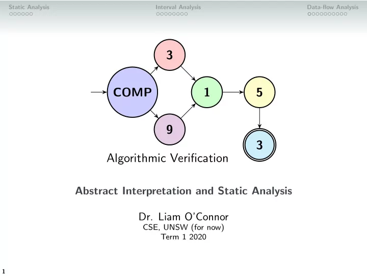
3 COMP 1 5 9 3 Algorithmic Verification Abstract - PowerPoint PPT Presentation
<latexit
Static Analysis Interval Analysis Data-flow Analysis Knaster-Tarski Theorem Let’s prove it for greatest fixed points, given a lattice L and a monotone function f : Define D = { x ∈ L | x � f ( x ) } . We know that ∀ m . ⊥ � m , so we know ⊥ ∈ D ,and, by monotonicity, f ( ⊥ ) ∈ D , f ( f ( ⊥ )) ∈ D etc. Let u = sup D , the least upper bound. Hence for all x ∈ D , x � u , and by monotonicity f ( x ) � f ( u ). Thus x � f ( x ) � f ( u ). So f ( u ) is also an upper bound of D . u is the least upper bound of D , so u � f ( u ). Thus u ∈ D . 20
Static Analysis Interval Analysis Data-flow Analysis Knaster-Tarski Theorem Let’s prove it for greatest fixed points, given a lattice L and a monotone function f : Define D = { x ∈ L | x � f ( x ) } . We know that ∀ m . ⊥ � m , so we know ⊥ ∈ D ,and, by monotonicity, f ( ⊥ ) ∈ D , f ( f ( ⊥ )) ∈ D etc. Let u = sup D , the least upper bound. Hence for all x ∈ D , x � u , and by monotonicity f ( x ) � f ( u ). Thus x � f ( x ) � f ( u ). So f ( u ) is also an upper bound of D . u is the least upper bound of D , so u � f ( u ). Thus u ∈ D . By monotonicity, f ( u ) � f ( f ( u )), 21
Static Analysis Interval Analysis Data-flow Analysis Knaster-Tarski Theorem Let’s prove it for greatest fixed points, given a lattice L and a monotone function f : Define D = { x ∈ L | x � f ( x ) } . We know that ∀ m . ⊥ � m , so we know ⊥ ∈ D ,and, by monotonicity, f ( ⊥ ) ∈ D , f ( f ( ⊥ )) ∈ D etc. Let u = sup D , the least upper bound. Hence for all x ∈ D , x � u , and by monotonicity f ( x ) � f ( u ). Thus x � f ( x ) � f ( u ). So f ( u ) is also an upper bound of D . u is the least upper bound of D , so u � f ( u ). Thus u ∈ D . By monotonicity, f ( u ) � f ( f ( u )), so f ( u ) ∈ D 22
Static Analysis Interval Analysis Data-flow Analysis Knaster-Tarski Theorem Let’s prove it for greatest fixed points, given a lattice L and a monotone function f : Define D = { x ∈ L | x � f ( x ) } . We know that ∀ m . ⊥ � m , so we know ⊥ ∈ D ,and, by monotonicity, f ( ⊥ ) ∈ D , f ( f ( ⊥ )) ∈ D etc. Let u = sup D , the least upper bound. Hence for all x ∈ D , x � u , and by monotonicity f ( x ) � f ( u ). Thus x � f ( x ) � f ( u ). So f ( u ) is also an upper bound of D . u is the least upper bound of D , so u � f ( u ). Thus u ∈ D . By monotonicity, f ( u ) � f ( f ( u )), so f ( u ) ∈ D Because u is the least upper bound of D , f ( u ) ≤ u . 23
Static Analysis Interval Analysis Data-flow Analysis Knaster-Tarski Theorem Let’s prove it for greatest fixed points, given a lattice L and a monotone function f : Define D = { x ∈ L | x � f ( x ) } . We know that ∀ m . ⊥ � m , so we know ⊥ ∈ D ,and, by monotonicity, f ( ⊥ ) ∈ D , f ( f ( ⊥ )) ∈ D etc. Let u = sup D , the least upper bound. Hence for all x ∈ D , x � u , and by monotonicity f ( x ) � f ( u ). Thus x � f ( x ) � f ( u ). So f ( u ) is also an upper bound of D . u is the least upper bound of D , so u � f ( u ). Thus u ∈ D . By monotonicity, f ( u ) � f ( f ( u )), so f ( u ) ∈ D Because u is the least upper bound of D , f ( u ) ≤ u . Therefore f ( u ) = u , i.e. u is a fixed point. 24
Static Analysis Interval Analysis Data-flow Analysis Knaster-Tarski Theorem Let’s prove it for greatest fixed points, given a lattice L and a monotone function f : Define D = { x ∈ L | x � f ( x ) } . We know that ∀ m . ⊥ � m , so we know ⊥ ∈ D ,and, by monotonicity, f ( ⊥ ) ∈ D , f ( f ( ⊥ )) ∈ D etc. Let u = sup D , the least upper bound. Hence for all x ∈ D , x � u , and by monotonicity f ( x ) � f ( u ). Thus x � f ( x ) � f ( u ). So f ( u ) is also an upper bound of D . u is the least upper bound of D , so u � f ( u ). Thus u ∈ D . By monotonicity, f ( u ) � f ( f ( u )), so f ( u ) ∈ D Because u is the least upper bound of D , f ( u ) ≤ u . Therefore f ( u ) = u , i.e. u is a fixed point. All fixed points are in D , therefore u is the greatest fixed point. 25
Static Analysis Interval Analysis Data-flow Analysis Fixed Point How do we compute fixed points? 26
Static Analysis Interval Analysis Data-flow Analysis Fixed Point How do we compute fixed points? For finite lattices , we can compute the least fixed point by iterating f from ⊥ , and the greatest by iterating from ⊤ : Let ι ∈ {⊤ , ⊥} depending on which fixed point we want: prev := ι curr := f ( prev ) while curr � = prev do prev := curr curr := f ( curr ) od 27
Static Analysis Interval Analysis Data-flow Analysis Fixed Point How do we compute fixed points? For finite lattices , we can compute the least fixed point by iterating f from ⊥ , and the greatest by iterating from ⊤ : Let ι ∈ {⊤ , ⊥} depending on which fixed point we want: prev := ι curr := f ( prev ) while curr � = prev do prev := curr curr := f ( curr ) od Why does this terminate? 28
Static Analysis Interval Analysis Data-flow Analysis Abstract Interpretation A very common use-case for fixed point computations is in abstract interpretation , a type of static analysis. Key Idea Replace concrete variables with approximate abstractions in 1 an abstract domain , which is a lattice. 29
Static Analysis Interval Analysis Data-flow Analysis Abstract Interpretation A very common use-case for fixed point computations is in abstract interpretation , a type of static analysis. Key Idea Replace concrete variables with approximate abstractions in 1 an abstract domain , which is a lattice. Approximate the program’s semantics using monotonic 2 functions defined over that domain. 30
Static Analysis Interval Analysis Data-flow Analysis Abstract Interpretation A very common use-case for fixed point computations is in abstract interpretation , a type of static analysis. Key Idea Replace concrete variables with approximate abstractions in 1 an abstract domain , which is a lattice. Approximate the program’s semantics using monotonic 2 functions defined over that domain. Compute the least fixed point of these functions. 3 31
Static Analysis Interval Analysis Data-flow Analysis Abstract Interpretation A very common use-case for fixed point computations is in abstract interpretation , a type of static analysis. Key Idea Replace concrete variables with approximate abstractions in 1 an abstract domain , which is a lattice. Approximate the program’s semantics using monotonic 2 functions defined over that domain. Compute the least fixed point of these functions. 3 We have seen this before. Predicate abstraction is an example of abstract interpretation. 32
Static Analysis Interval Analysis Data-flow Analysis The WHILE Language To make things easier, we will define a simple imperative programming language as follows: A ::= � arithmetic expressions � B � boolean expressions � ::= [ x := A ] ℓ | [ skip ] ℓ | S 1 ; S 2 S ::= if [ B ] ℓ then S else S | while [ B ] ℓ do S | Note that we label all statements and conditions (usually with a number). These labelled terms correspond to nodes on the control flow graph. 33
Static Analysis Interval Analysis Data-flow Analysis Examples if [ x > 0] 1 then [ x := 2 x + 1] 2 else [ x := 1 − 4 x ] 3 [ x := 8 ÷ x ] 4
Static Analysis Interval Analysis Data-flow Analysis Examples if [ x > 0] 1 then [ x > 0] 1 [ x := 2 x + 1] 2 else [ x := 1 − 4 x ] 3 [ x := 2 x + 1] 2 [ x := 1 − 4 x ] 3 [ x := 8 ÷ x ] 4 [ x := 8 ÷ x ] 4
Static Analysis Interval Analysis Data-flow Analysis Examples if [ x > 0] 1 then [ x > 0] 1 [ x := 2 x + 1] 2 else [ x := 1 − 4 x ] 3 [ x := 2 x + 1] 2 [ x := 1 − 4 x ] 3 [ x := 8 ÷ x ] 4 [ x := 8 ÷ x ] 4 What abstract domain should we use to detect divide by zero? 36
Static Analysis Interval Analysis Data-flow Analysis Intervals Let’s define intervals n , m as either: ∅ , the empty interval, or [ n , m ] where n , m ∈ Z ∪ { + ∞ , −∞} . 37
Static Analysis Interval Analysis Data-flow Analysis Intervals Let’s define intervals n , m as either: ∅ , the empty interval, or [ n , m ] where n , m ∈ Z ∪ { + ∞ , −∞} . We can define interval intersection n ∩ m as the interval where n and m overlap. 38
Static Analysis Interval Analysis Data-flow Analysis Intervals Let’s define intervals n , m as either: ∅ , the empty interval, or [ n , m ] where n , m ∈ Z ∪ { + ∞ , −∞} . We can define interval intersection n ∩ m as the interval where n and m overlap. Likewise, define union n ∪ m as the smallest interval containing both n and m . 39
Static Analysis Interval Analysis Data-flow Analysis Intervals Let’s define intervals n , m as either: ∅ , the empty interval, or [ n , m ] where n , m ∈ Z ∪ { + ∞ , −∞} . We can define interval intersection n ∩ m as the interval where n and m overlap. Likewise, define union n ∪ m as the smallest interval containing both n and m . Observation Define inf S = � S and sup S = � S , then intervals form a lattice: ⊥ = ∅ and ⊤ = [ −∞ , + ∞ ]. The ordering � here is interval inclusion. 40
Static Analysis Interval Analysis Data-flow Analysis Intervals Let’s define intervals n , m as either: ∅ , the empty interval, or [ n , m ] where n , m ∈ Z ∪ { + ∞ , −∞} . We can define interval intersection n ∩ m as the interval where n and m overlap. Likewise, define union n ∪ m as the smallest interval containing both n and m . Observation Define inf S = � S and sup S = � S , then intervals form a lattice: ⊥ = ∅ and ⊤ = [ −∞ , + ∞ ]. The ordering � here is interval inclusion. We can “lift” arithmetic operators to the interval level, where they apply to both bounds. Similarly define e.g. ˆ 3 = [3 , 3]. 41
Static Analysis Interval Analysis Data-flow Analysis Equation Systems We define a series of entry interval equations x i , and a series of exit equations x ′ i describing the possible values of x before and after the statement i . [ x > 0] 1 x 1 = [ x := 2 x + 1] 2 [ x := 1 − 4 x ] 3 [ x := 8 ÷ x ] 4
Static Analysis Interval Analysis Data-flow Analysis Equation Systems We define a series of entry interval equations x i , and a series of exit equations x ′ i describing the possible values of x before and after the statement i . [ x > 0] 1 x 1 = [ −∞ , + ∞ ] x ′ = 1 [ x := 2 x + 1] 2 [ x := 1 − 4 x ] 3 [ x := 8 ÷ x ] 4
Static Analysis Interval Analysis Data-flow Analysis Equation Systems We define a series of entry interval equations x i , and a series of exit equations x ′ i describing the possible values of x before and after the statement i . [ x > 0] 1 x 1 = [ −∞ , + ∞ ] x ′ = x 1 1 = x 2 [ x := 2 x + 1] 2 [ x := 1 − 4 x ] 3 [ x := 8 ÷ x ] 4
Static Analysis Interval Analysis Data-flow Analysis Equation Systems We define a series of entry interval equations x i , and a series of exit equations x ′ i describing the possible values of x before and after the statement i . [ x > 0] 1 x 1 = [ −∞ , + ∞ ] x ′ = x 1 1 x ′ = 1 ∩ [1 , + ∞ ] x 2 x ′ = [ x := 2 x + 1] 2 [ x := 1 − 4 x ] 3 2 [ x := 8 ÷ x ] 4
Static Analysis Interval Analysis Data-flow Analysis Equation Systems We define a series of entry interval equations x i , and a series of exit equations x ′ i describing the possible values of x before and after the statement i . [ x > 0] 1 x 1 = [ −∞ , + ∞ ] x ′ = x 1 1 x ′ = 1 ∩ [1 , + ∞ ] x 2 ˆ 2 × x 2 + ˆ x ′ = 1 [ x := 2 x + 1] 2 [ x := 1 − 4 x ] 3 2 x 3 = [ x := 8 ÷ x ] 4
Static Analysis Interval Analysis Data-flow Analysis Equation Systems We define a series of entry interval equations x i , and a series of exit equations x ′ i describing the possible values of x before and after the statement i . [ x > 0] 1 x 1 = [ −∞ , + ∞ ] x ′ = x 1 1 x ′ = 1 ∩ [1 , + ∞ ] x 2 2 × x 2 + ˆ ˆ x ′ = 1 [ x := 2 x + 1] 2 [ x := 1 − 4 x ] 3 2 x ′ 1 ∩ [ −∞ , 0] x 3 = x ′ = 3 [ x := 8 ÷ x ] 4
Static Analysis Interval Analysis Data-flow Analysis Equation Systems We define a series of entry interval equations x i , and a series of exit equations x ′ i describing the possible values of x before and after the statement i . [ x > 0] 1 x 1 = [ −∞ , + ∞ ] x ′ = x 1 1 x ′ = 1 ∩ [1 , + ∞ ] x 2 ˆ 2 × x 2 + ˆ x ′ = 1 [ x := 2 x + 1] 2 [ x := 1 − 4 x ] 3 2 x ′ 1 ∩ [ −∞ , 0] x 3 = ˆ 1 − ˆ x ′ 4 × x 3 = 3 = x 4 [ x := 8 ÷ x ] 4
Static Analysis Interval Analysis Data-flow Analysis Equation Systems We define a series of entry interval equations x i , and a series of exit equations x ′ i describing the possible values of x before and after the statement i . [ x > 0] 1 x 1 = [ −∞ , + ∞ ] x ′ = x 1 1 x ′ = 1 ∩ [1 , + ∞ ] x 2 ˆ 2 × x 2 + ˆ x ′ = 1 [ x := 2 x + 1] 2 [ x := 1 − 4 x ] 3 2 x ′ 1 ∩ [ −∞ , 0] x 3 = ˆ 1 − ˆ x ′ 4 × x 3 = 3 x ′ 2 ∪ x ′ = x 4 [ x := 8 ÷ x ] 4 3 x ′ = 4
Static Analysis Interval Analysis Data-flow Analysis Equation Systems We define a series of entry interval equations x i , and a series of exit equations x ′ i describing the possible values of x before and after the statement i . [ x > 0] 1 x 1 = [ −∞ , + ∞ ] x ′ = x 1 1 x ′ = 1 ∩ [1 , + ∞ ] x 2 2 × x 2 + ˆ ˆ x ′ = 1 [ x := 2 x + 1] 2 [ x := 1 − 4 x ] 3 2 x ′ 1 ∩ [ −∞ , 0] x 3 = ˆ 1 − ˆ x ′ 4 × x 3 = 3 x ′ 2 ∪ x ′ = x 4 [ x := 8 ÷ x ] 4 3 ˆ x ′ = 8 ÷ x 4 4
Static Analysis Interval Analysis Data-flow Analysis Equation Systems We define a series of entry interval equations x i , and a series of exit equations x ′ i describing the possible values of x before and after the statement i . [ x > 0] 1 x 1 = [ −∞ , + ∞ ] x ′ = x 1 1 x ′ = 1 ∩ [1 , + ∞ ] x 2 2 × x 2 + ˆ ˆ x ′ = 1 [ x := 2 x + 1] 2 [ x := 1 − 4 x ] 3 2 x ′ 1 ∩ [ −∞ , 0] x 3 = ˆ 1 − ˆ x ′ 4 × x 3 = 3 x ′ 2 ∪ x ′ = x 4 [ x := 8 ÷ x ] 4 3 ˆ x ′ = 8 ÷ x 4 4 Observe that all operations used are monotone. How can we compute what the intervals are? Iterate to the least fixed point ! 51
Static Analysis Interval Analysis Data-flow Analysis Least Fixed Points for Equation Systems We start initialising all equations to ⊥ , and then iterate until the results stop changing. We can choose the equations in any (fair) order, and we will always reach a fixed point eventually. Some ways are faster than others. ∅ [ −∞ , + ∞ ] x 1 = = x ′ = ∅ = x 1 1 x ′ ∅ 1 ∩ [1 , + ∞ ] x 2 = = ˆ 2 × x 2 + ˆ x ′ ∅ = = 1 2 x ′ = ∅ = 1 ∩ [ −∞ , 0] x 3 1 − ˆ ˆ x ′ = ∅ = 4 × x 3 3 x ′ 2 ∪ x ′ ∅ x 4 = = 3 ˆ x ′ ∅ 8 ÷ x 4 = = 4 52
Static Analysis Interval Analysis Data-flow Analysis Least Fixed Points for Equation Systems We start initialising all equations to ⊥ , and then iterate until the results stop changing. We can choose the equations in any (fair) order, and we will always reach a fixed point eventually. Some ways are faster than others. ∅ = [ −∞ , + ∞ ] [ −∞ , + ∞ ] x 1 = = x ′ = ∅ = x 1 1 x ′ ∅ 1 ∩ [1 , + ∞ ] x 2 = = ˆ 2 × x 2 + ˆ x ′ ∅ = = 1 2 x ′ = ∅ = 1 ∩ [ −∞ , 0] x 3 1 − ˆ ˆ x ′ = ∅ = 4 × x 3 3 x ′ 2 ∪ x ′ ∅ x 4 = = 3 ˆ x ′ ∅ 8 ÷ x 4 = = 4 53
Static Analysis Interval Analysis Data-flow Analysis Least Fixed Points for Equation Systems We start initialising all equations to ⊥ , and then iterate until the results stop changing. We can choose the equations in any (fair) order, and we will always reach a fixed point eventually. Some ways are faster than others. ∅ = [ −∞ , + ∞ ] [ −∞ , + ∞ ] x 1 = = x ′ = ∅ = [ −∞ , + ∞ ] = x 1 1 x ′ ∅ 1 ∩ [1 , + ∞ ] x 2 = = ˆ 2 × x 2 + ˆ x ′ ∅ = = 1 2 x ′ = ∅ = 1 ∩ [ −∞ , 0] x 3 1 − ˆ ˆ x ′ = ∅ = 4 × x 3 3 x ′ 2 ∪ x ′ ∅ x 4 = = 3 ˆ x ′ ∅ 8 ÷ x 4 = = 4 54
Static Analysis Interval Analysis Data-flow Analysis Least Fixed Points for Equation Systems We start initialising all equations to ⊥ , and then iterate until the results stop changing. We can choose the equations in any (fair) order, and we will always reach a fixed point eventually. Some ways are faster than others. ∅ = [ −∞ , + ∞ ] [ −∞ , + ∞ ] x 1 = = x ′ = ∅ = [ −∞ , + ∞ ] = x 1 1 x ′ ∅ = [1 , + ∞ ] 1 ∩ [1 , + ∞ ] x 2 = = ˆ 2 × x 2 + ˆ x ′ ∅ = = 1 2 x ′ = ∅ = 1 ∩ [ −∞ , 0] x 3 1 − ˆ ˆ x ′ = ∅ = 4 × x 3 3 x ′ 2 ∪ x ′ ∅ x 4 = = 3 ˆ x ′ ∅ 8 ÷ x 4 = = 4 55
Static Analysis Interval Analysis Data-flow Analysis Least Fixed Points for Equation Systems We start initialising all equations to ⊥ , and then iterate until the results stop changing. We can choose the equations in any (fair) order, and we will always reach a fixed point eventually. Some ways are faster than others. ∅ = [ −∞ , + ∞ ] [ −∞ , + ∞ ] x 1 = = x ′ = ∅ = [ −∞ , + ∞ ] = x 1 1 x ′ ∅ = [1 , + ∞ ] 1 ∩ [1 , + ∞ ] x 2 = = ˆ 2 × x 2 + ˆ x ′ ∅ = [3 , + ∞ ] = = 1 2 x ′ = ∅ = 1 ∩ [ −∞ , 0] x 3 1 − ˆ ˆ x ′ = ∅ = 4 × x 3 3 x ′ 2 ∪ x ′ ∅ x 4 = = 3 ˆ x ′ ∅ 8 ÷ x 4 = = 4 56
Static Analysis Interval Analysis Data-flow Analysis Least Fixed Points for Equation Systems We start initialising all equations to ⊥ , and then iterate until the results stop changing. We can choose the equations in any (fair) order, and we will always reach a fixed point eventually. Some ways are faster than others. ∅ = [ −∞ , + ∞ ] [ −∞ , + ∞ ] x 1 = = x ′ = ∅ = [ −∞ , + ∞ ] = x 1 1 x ′ ∅ = [1 , + ∞ ] 1 ∩ [1 , + ∞ ] x 2 = = ˆ 2 × x 2 + ˆ x ′ ∅ = [3 , + ∞ ] = = 1 2 x ′ = ∅ = [ −∞ , 0] = 1 ∩ [ −∞ , 0] x 3 1 − ˆ ˆ x ′ = ∅ = 4 × x 3 3 x ′ 2 ∪ x ′ ∅ x 4 = = 3 ˆ x ′ ∅ 8 ÷ x 4 = = 4 57
Static Analysis Interval Analysis Data-flow Analysis Least Fixed Points for Equation Systems We start initialising all equations to ⊥ , and then iterate until the results stop changing. We can choose the equations in any (fair) order, and we will always reach a fixed point eventually. Some ways are faster than others. ∅ = [ −∞ , + ∞ ] [ −∞ , + ∞ ] x 1 = = x ′ = ∅ = [ −∞ , + ∞ ] = x 1 1 x ′ ∅ = [1 , + ∞ ] 1 ∩ [1 , + ∞ ] x 2 = = ˆ 2 × x 2 + ˆ x ′ ∅ = [3 , + ∞ ] = = 1 2 x ′ = ∅ = [ −∞ , 0] = 1 ∩ [ −∞ , 0] x 3 1 − ˆ ˆ x ′ = ∅ = [1 , + ∞ ] = 4 × x 3 3 x ′ 2 ∪ x ′ ∅ x 4 = = 3 ˆ x ′ ∅ 8 ÷ x 4 = = 4 58
Static Analysis Interval Analysis Data-flow Analysis Least Fixed Points for Equation Systems We start initialising all equations to ⊥ , and then iterate until the results stop changing. We can choose the equations in any (fair) order, and we will always reach a fixed point eventually. Some ways are faster than others. ∅ = [ −∞ , + ∞ ] [ −∞ , + ∞ ] x 1 = = x ′ = ∅ = [ −∞ , + ∞ ] = x 1 1 x ′ ∅ = [1 , + ∞ ] 1 ∩ [1 , + ∞ ] x 2 = = ˆ 2 × x 2 + ˆ x ′ ∅ = [3 , + ∞ ] = = 1 2 x ′ = ∅ = [ −∞ , 0] = 1 ∩ [ −∞ , 0] x 3 1 − ˆ ˆ x ′ = ∅ = [1 , + ∞ ] = 4 × x 3 3 x ′ 2 ∪ x ′ ∅ = [1 , + ∞ ] x 4 = = 3 ˆ x ′ ∅ 8 ÷ x 4 = = 4 59
Static Analysis Interval Analysis Data-flow Analysis Least Fixed Points for Equation Systems We start initialising all equations to ⊥ , and then iterate until the results stop changing. We can choose the equations in any (fair) order, and we will always reach a fixed point eventually. Some ways are faster than others. ∅ = [ −∞ , + ∞ ] [ −∞ , + ∞ ] x 1 = = x ′ = ∅ = [ −∞ , + ∞ ] = x 1 1 x ′ ∅ = [1 , + ∞ ] 1 ∩ [1 , + ∞ ] x 2 = = ˆ 2 × x 2 + ˆ x ′ ∅ = [3 , + ∞ ] = = 1 2 x ′ = ∅ = [ −∞ , 0] = 1 ∩ [ −∞ , 0] x 3 1 − ˆ ˆ x ′ = ∅ = [1 , + ∞ ] = 4 × x 3 3 x ′ 2 ∪ x ′ ∅ = [1 , + ∞ ] x 4 = = 3 ˆ x ′ ∅ = [0 , 8] 8 ÷ x 4 = = 4 60
Static Analysis Interval Analysis Data-flow Analysis Least Fixed Points for Equation Systems We start initialising all equations to ⊥ , and then iterate until the results stop changing. We can choose the equations in any (fair) order, and we will always reach a fixed point eventually. Some ways are faster than others. ∅ = [ −∞ , + ∞ ] [ −∞ , + ∞ ] x 1 = = x ′ = ∅ = [ −∞ , + ∞ ] = x 1 1 x ′ ∅ = [1 , + ∞ ] 1 ∩ [1 , + ∞ ] x 2 = = 2 × x 2 + ˆ ˆ x ′ ∅ = [3 , + ∞ ] = = 1 2 x ′ = ∅ = [ −∞ , 0] = 1 ∩ [ −∞ , 0] x 3 ˆ 1 − ˆ x ′ = ∅ = [1 , + ∞ ] = 4 × x 3 3 x ′ 2 ∪ x ′ ∅ = [1 , + ∞ ] x 4 = = 3 ˆ x ′ ∅ = [0 , 8] 8 ÷ x 4 = = 4 Seeing as 0 / ∈ x 4 , we know divide by zero is impossible. 61
Static Analysis Interval Analysis Data-flow Analysis Slow Convergence Because the previous example had no loops, all equations converged after one step. Compare to this example: [ n := 1] 1 while [ n < 1000] 2 do [ n := n + 1] 3 [ skip ] 4 Slightly simplified equations for presentation: n ′ = ∅ = [1 , 1] 1 n ′ 1 ∪ n ′ ∅ n 2 = = 3 = ∅ = n 2 ∩ [ −∞ , 999] n 3 n ′ ∅ = = n 3 + 1 3 n ′ = ∅ = 3 ∩ [1000 , + ∞ ] n 4 62
Static Analysis Interval Analysis Data-flow Analysis Slow Convergence Because the previous example had no loops, all equations converged after one step. Compare to this example: [ n := 1] 1 while [ n < 1000] 2 do [ n := n + 1] 3 [ skip ] 4 Slightly simplified equations for presentation: n ′ = ∅ = [1 , 1] = [1 , 1] 1 n ′ 1 ∪ n ′ ∅ n 2 = = 3 = ∅ = n 2 ∩ [ −∞ , 999] n 3 n ′ ∅ = = n 3 + 1 3 n ′ = ∅ = 3 ∩ [1000 , + ∞ ] n 4 63
Static Analysis Interval Analysis Data-flow Analysis Slow Convergence Because the previous example had no loops, all equations converged after one step. Compare to this example: [ n := 1] 1 while [ n < 1000] 2 do [ n := n + 1] 3 [ skip ] 4 Slightly simplified equations for presentation: n ′ = ∅ = [1 , 1] = [1 , 1] 1 n ′ 1 ∪ n ′ ∅ = [1 , 1] n 2 = = 3 = ∅ = n 2 ∩ [ −∞ , 999] n 3 n ′ ∅ = = n 3 + 1 3 n ′ = ∅ = 3 ∩ [1000 , + ∞ ] n 4 64
Static Analysis Interval Analysis Data-flow Analysis Slow Convergence Because the previous example had no loops, all equations converged after one step. Compare to this example: [ n := 1] 1 while [ n < 1000] 2 do [ n := n + 1] 3 [ skip ] 4 Slightly simplified equations for presentation: n ′ = ∅ = [1 , 1] = [1 , 1] 1 n ′ 1 ∪ n ′ ∅ = [1 , 1] n 2 = = 3 = ∅ = [1 , 1] = n 2 ∩ [ −∞ , 999] n 3 n ′ ∅ = = n 3 + 1 3 n ′ = ∅ = 3 ∩ [1000 , + ∞ ] n 4 65
Static Analysis Interval Analysis Data-flow Analysis Slow Convergence Because the previous example had no loops, all equations converged after one step. Compare to this example: [ n := 1] 1 while [ n < 1000] 2 do [ n := n + 1] 3 [ skip ] 4 Slightly simplified equations for presentation: n ′ = ∅ = [1 , 1] = [1 , 1] 1 n ′ 1 ∪ n ′ ∅ = [1 , 1] n 2 = = 3 = ∅ = [1 , 1] = n 2 ∩ [ −∞ , 999] n 3 n ′ ∅ = [2 , 2] = = n 3 + 1 3 n ′ = ∅ = 3 ∩ [1000 , + ∞ ] n 4 66
Static Analysis Interval Analysis Data-flow Analysis Slow Convergence Because the previous example had no loops, all equations converged after one step. Compare to this example: [ n := 1] 1 while [ n < 1000] 2 do [ n := n + 1] 3 [ skip ] 4 Slightly simplified equations for presentation: n ′ = ∅ = [1 , 1] = [1 , 1] 1 n ′ 1 ∪ n ′ ∅ = [1 , 1] = [1 , 2] n 2 = = 3 = ∅ = [1 , 1] = n 2 ∩ [ −∞ , 999] n 3 n ′ ∅ = [2 , 2] = = n 3 + 1 3 n ′ = ∅ = 3 ∩ [1000 , + ∞ ] n 4 67
Static Analysis Interval Analysis Data-flow Analysis Slow Convergence Because the previous example had no loops, all equations converged after one step. Compare to this example: [ n := 1] 1 while [ n < 1000] 2 do [ n := n + 1] 3 [ skip ] 4 Slightly simplified equations for presentation: n ′ = ∅ = [1 , 1] = [1 , 1] 1 n ′ 1 ∪ n ′ ∅ = [1 , 1] = [1 , 2] n 2 = = 3 = ∅ = [1 , 1] = [1 , 2] = n 2 ∩ [ −∞ , 999] n 3 n ′ ∅ = [2 , 2] = = n 3 + 1 3 n ′ = ∅ = 3 ∩ [1000 , + ∞ ] n 4 68
Static Analysis Interval Analysis Data-flow Analysis Slow Convergence Because the previous example had no loops, all equations converged after one step. Compare to this example: [ n := 1] 1 while [ n < 1000] 2 do [ n := n + 1] 3 [ skip ] 4 Slightly simplified equations for presentation: n ′ = ∅ = [1 , 1] = [1 , 1] 1 n ′ 1 ∪ n ′ ∅ = [1 , 1] = [1 , 2] n 2 = = 3 = ∅ = [1 , 1] = [1 , 2] = n 2 ∩ [ −∞ , 999] n 3 n ′ ∅ = [2 , 2] = [2 , 3] = = n 3 + 1 3 n ′ = ∅ = 3 ∩ [1000 , + ∞ ] n 4 69
Static Analysis Interval Analysis Data-flow Analysis Slow Convergence Because the previous example had no loops, all equations converged after one step. Compare to this example: [ n := 1] 1 while [ n < 1000] 2 do [ n := n + 1] 3 [ skip ] 4 Slightly simplified equations for presentation: n ′ = ∅ = [1 , 1] = [1 , 1] 1 n ′ 1 ∪ n ′ ∅ = [1 , 1] = [1 , 2] = [1 , 3] n 2 = = 3 = ∅ = [1 , 1] = [1 , 2] = n 2 ∩ [ −∞ , 999] n 3 n ′ ∅ = [2 , 2] = [2 , 3] = = n 3 + 1 3 n ′ = ∅ = 3 ∩ [1000 , + ∞ ] n 4 70
Static Analysis Interval Analysis Data-flow Analysis Slow Convergence Because the previous example had no loops, all equations converged after one step. Compare to this example: [ n := 1] 1 while [ n < 1000] 2 do [ n := n + 1] 3 [ skip ] 4 Slightly simplified equations for presentation: n ′ = ∅ = [1 , 1] = [1 , 1] 1 n ′ 1 ∪ n ′ ∅ = [1 , 1] = [1 , 2] = [1 , 3] n 2 = = 3 = ∅ = [1 , 1] = [1 , 2] = [1 , 3] = n 2 ∩ [ −∞ , 999] n 3 n ′ ∅ = [2 , 2] = [2 , 3] = = n 3 + 1 3 n ′ = ∅ = 3 ∩ [1000 , + ∞ ] n 4 71
Static Analysis Interval Analysis Data-flow Analysis Slow Convergence Because the previous example had no loops, all equations converged after one step. Compare to this example: [ n := 1] 1 while [ n < 1000] 2 do [ n := n + 1] 3 [ skip ] 4 Slightly simplified equations for presentation: n ′ = ∅ = [1 , 1] = [1 , 1] 1 n ′ 1 ∪ n ′ ∅ = [1 , 1] = [1 , 2] = [1 , 3] = · · · n 2 = = 3 = ∅ = [1 , 1] = [1 , 2] = [1 , 3] = · · · = n 2 ∩ [ −∞ , 999] n 3 n ′ ∅ = [2 , 2] = [2 , 3] = [2 , 4] = · · · = = n 3 + 1 3 n ′ = ∅ = 3 ∩ [1000 , + ∞ ] n 4 This is going to take a long time to converge! (1000 steps) 72
Static Analysis Interval Analysis Data-flow Analysis Widening Our interval abstraction is too detailed, making our loop iterations take ages. 73
Static Analysis Interval Analysis Data-flow Analysis Widening Our interval abstraction is too detailed, making our loop iterations take ages. Solution Let n be the value we are updating and m be the result of the next iteration. Then, we update with n ▽ m instead of m : ∅ ▽ m = m n ▽ ∅ = n [ if ℓ 1 < ℓ 0 then − ∞ else ℓ 1 [ ℓ 0 , u 0 ] ▽ [ ℓ 1 , u 1 ] = , if u 1 > u 0 then + ∞ else u 1 ] In other words, if we ever try to loosen a bound, we just extrapolate all the way to infinity. 74
Static Analysis Interval Analysis Data-flow Analysis Widening Our interval abstraction is too detailed, making our loop iterations take ages. Solution Let n be the value we are updating and m be the result of the next iteration. Then, we update with n ▽ m instead of m : ∅ ▽ m = m n ▽ ∅ = n [ if ℓ 1 < ℓ 0 then − ∞ else ℓ 1 [ ℓ 0 , u 0 ] ▽ [ ℓ 1 , u 1 ] = , if u 1 > u 0 then + ∞ else u 1 ] In other words, if we ever try to loosen a bound, we just extrapolate all the way to infinity. This is an overapproximation, but it converges much faster than the normal iterative sequence does. 75
Static Analysis Interval Analysis Data-flow Analysis Loops with Widening n ′ = ∅ = [1 , 1] 1 n ′ 1 ∪ n ′ = ∅ = n 2 3 n 3 = ∅ = n 2 ∩ [ −∞ , 999] n ′ = ∅ = n 3 + 1 3 n ′ n 4 = ∅ = 3 ∩ [1000 , + ∞ ] 76
Static Analysis Interval Analysis Data-flow Analysis Loops with Widening n ′ = ∅ = [1 , 1] = [1 , 1] 1 n ′ 1 ∪ n ′ = ∅ = n 2 3 n 3 = ∅ = n 2 ∩ [ −∞ , 999] n ′ = ∅ = n 3 + 1 3 n ′ n 4 = ∅ = 3 ∩ [1000 , + ∞ ] 77
Static Analysis Interval Analysis Data-flow Analysis Loops with Widening n ′ = ∅ = [1 , 1] = [1 , 1] 1 n ′ 1 ∪ n ′ = ∅ = [1 , 1] = n 2 3 n 3 = ∅ = n 2 ∩ [ −∞ , 999] n ′ = ∅ = n 3 + 1 3 n ′ n 4 = ∅ = 3 ∩ [1000 , + ∞ ] 78
Static Analysis Interval Analysis Data-flow Analysis Loops with Widening n ′ = ∅ = [1 , 1] = [1 , 1] 1 n ′ 1 ∪ n ′ = ∅ = [1 , 1] = n 2 3 n 3 = ∅ = [1 , 1] = n 2 ∩ [ −∞ , 999] n ′ = ∅ = n 3 + 1 3 n ′ n 4 = ∅ = 3 ∩ [1000 , + ∞ ] 79
Static Analysis Interval Analysis Data-flow Analysis Loops with Widening n ′ = ∅ = [1 , 1] = [1 , 1] 1 n ′ 1 ∪ n ′ = ∅ = [1 , 1] = n 2 3 n 3 = ∅ = [1 , 1] = n 2 ∩ [ −∞ , 999] n ′ = ∅ = [2 , 2] = n 3 + 1 3 n ′ n 4 = ∅ = 3 ∩ [1000 , + ∞ ] 80
Static Analysis Interval Analysis Data-flow Analysis Loops with Widening n ′ = ∅ = [1 , 1] = [1 , 1] 1 n ′ 1 ∪ n ′ = ∅ = [1 , 1] = [1 , + ∞ ] = n 2 3 n 3 = ∅ = [1 , 1] = n 2 ∩ [ −∞ , 999] n ′ = ∅ = [2 , 2] = n 3 + 1 3 n ′ n 4 = ∅ = 3 ∩ [1000 , + ∞ ] 81
Static Analysis Interval Analysis Data-flow Analysis Loops with Widening n ′ = ∅ = [1 , 1] = [1 , 1] 1 n ′ 1 ∪ n ′ = ∅ = [1 , 1] = [1 , + ∞ ] = n 2 3 n 3 = ∅ = [1 , 1] = [1 , 999] = n 2 ∩ [ −∞ , 999] n ′ = ∅ = [2 , 2] = n 3 + 1 3 n ′ n 4 = ∅ = 3 ∩ [1000 , + ∞ ] 82
Static Analysis Interval Analysis Data-flow Analysis Loops with Widening n ′ = ∅ = [1 , 1] = [1 , 1] 1 n ′ 1 ∪ n ′ = ∅ = [1 , 1] = [1 , + ∞ ] = n 2 3 n 3 = ∅ = [1 , 1] = [1 , 999] = n 2 ∩ [ −∞ , 999] n ′ = ∅ = [2 , 2] = [2 , 1000] = n 3 + 1 3 n ′ n 4 = ∅ = 3 ∩ [1000 , + ∞ ] 83
Static Analysis Interval Analysis Data-flow Analysis Loops with Widening n ′ = ∅ = [1 , 1] = [1 , 1] 1 n ′ 1 ∪ n ′ = ∅ = [1 , 1] = [1 , + ∞ ] = [1 , 1000] = n 2 3 n 3 = ∅ = [1 , 1] = [1 , 999] = n 2 ∩ [ −∞ , 999] n ′ = ∅ = [2 , 2] = [2 , 1000] = n 3 + 1 3 n ′ n 4 = ∅ = 3 ∩ [1000 , + ∞ ] 84
Static Analysis Interval Analysis Data-flow Analysis Loops with Widening n ′ = ∅ = [1 , 1] = [1 , 1] 1 n ′ 1 ∪ n ′ = ∅ = [1 , 1] = [1 , + ∞ ] = [1 , 1000] = n 2 3 n 3 = ∅ = [1 , 1] = [1 , 999] = [1 , 999] = n 2 ∩ [ −∞ , 999] n ′ = ∅ = [2 , 2] = [2 , 1000] = n 3 + 1 3 n ′ n 4 = ∅ = 3 ∩ [1000 , + ∞ ] 85
Static Analysis Interval Analysis Data-flow Analysis Loops with Widening n ′ = ∅ = [1 , 1] = [1 , 1] 1 n ′ 1 ∪ n ′ = ∅ = [1 , 1] = [1 , + ∞ ] = [1 , 1000] = n 2 3 n 3 = ∅ = [1 , 1] = [1 , 999] = [1 , 999] = n 2 ∩ [ −∞ , 999] n ′ = ∅ = [2 , 2] = [2 , 1000] = [2 , 1000] = n 3 + 1 3 n ′ n 4 = ∅ = 3 ∩ [1000 , + ∞ ] 86
Static Analysis Interval Analysis Data-flow Analysis Loops with Widening n ′ = ∅ = [1 , 1] = [1 , 1] 1 n ′ 1 ∪ n ′ = ∅ = [1 , 1] = [1 , + ∞ ] = [1 , 1000] = n 2 3 n 3 = ∅ = [1 , 1] = [1 , 999] = [1 , 999] = n 2 ∩ [ −∞ , 999] n ′ = ∅ = [2 , 2] = [2 , 1000] = [2 , 1000] = n 3 + 1 3 n ′ n 4 = ∅ = [1000 , 1000] = 3 ∩ [1000 , + ∞ ] 87
Static Analysis Interval Analysis Data-flow Analysis Beyond Interval Anaylsis Interval analysis is very effective but not very accurate, because it doesn’t express the relationships between variables. 88
Static Analysis Interval Analysis Data-flow Analysis Beyond Interval Anaylsis Interval analysis is very effective but not very accurate, because it doesn’t express the relationships between variables. Predicate abstraction and polyhedral models do better in many cases, but are more complicated. 89
Static Analysis Interval Analysis Data-flow Analysis Beyond Interval Anaylsis Interval analysis is very effective but not very accurate, because it doesn’t express the relationships between variables. Predicate abstraction and polyhedral models do better in many cases, but are more complicated. All are based on the same principle of least-fixed point of a system of equations. 90
Static Analysis Interval Analysis Data-flow Analysis Data-flow Analysis Data-flow analysis is a type of static analysis used extensively in compilers. 91
Static Analysis Interval Analysis Data-flow Analysis Data-flow Analysis Data-flow analysis is a type of static analysis used extensively in compilers. Example Available Expressions Analysis – Compute what expressions must have already been computed (and don’t need to be recomputed). 92
Static Analysis Interval Analysis Data-flow Analysis Data-flow Analysis Data-flow analysis is a type of static analysis used extensively in compilers. Example Available Expressions Analysis – Compute what expressions must have already been computed (and don’t need to be recomputed). Live Variables Analysis – Compute which variables may be read before next being written to (and thus hold important values). 93
Static Analysis Interval Analysis Data-flow Analysis Data-flow Analysis Data-flow analysis is a type of static analysis used extensively in compilers. Example Available Expressions Analysis – Compute what expressions must have already been computed (and don’t need to be recomputed). Live Variables Analysis – Compute which variables may be read before next being written to (and thus hold important values). Data-flow analyses may be forwards or backwards , and may or must . 94
Static Analysis Interval Analysis Data-flow Analysis Data-flow Analysis Data-flow analysis is a type of static analysis used extensively in compilers. Example Available Expressions Analysis – Compute what expressions must have already been computed (and don’t need to be recomputed). Live Variables Analysis – Compute which variables may be read before next being written to (and thus hold important values). Data-flow analyses may be forwards or backwards , and may or must . AEA is a forwards must analysis. 95
Static Analysis Interval Analysis Data-flow Analysis Data-flow Analysis Data-flow analysis is a type of static analysis used extensively in compilers. Example Available Expressions Analysis – Compute what expressions must have already been computed (and don’t need to be recomputed). Live Variables Analysis – Compute which variables may be read before next being written to (and thus hold important values). Data-flow analyses may be forwards or backwards , and may or must . AEA is a forwards must analysis. LVA is a backwards may analysis. 96
Static Analysis Interval Analysis Data-flow Analysis Step 1: Gen and Kill Each location in the CFG has an associated gen set, of generated information, and kill set, of information that is no longer accurate. 97
Static Analysis Interval Analysis Data-flow Analysis Step 1: Gen and Kill Each location in the CFG has an associated gen set, of generated information, and kill set, of information that is no longer accurate. Example (AEA) In AEA, gen AE ( ℓ ) is the expressions evaluated (and not updated) in ℓ and kill AE ( ℓ ) is those expressions updated by ℓ . 98
Static Analysis Interval Analysis Data-flow Analysis Step 1: Gen and Kill Each location in the CFG has an associated gen set, of generated information, and kill set, of information that is no longer accurate. Example (AEA) In AEA, gen AE ( ℓ ) is the expressions evaluated (and not updated) in ℓ and kill AE ( ℓ ) is those expressions updated by ℓ . For example, x := a + b would generate { a + b } , but kill any expression involving x . 99
Static Analysis Interval Analysis Data-flow Analysis Step 1: Gen and Kill Each location in the CFG has an associated gen set, of generated information, and kill set, of information that is no longer accurate. Example (AEA) In AEA, gen AE ( ℓ ) is the expressions evaluated (and not updated) in ℓ and kill AE ( ℓ ) is those expressions updated by ℓ . For example, x := a + b would generate { a + b } , but kill any expression involving x . Note : a := a + 1 would kill a + 1, not generate it. Why? Example (LVA) In LVA 100
Recommend
More recommend
Explore More Topics
Stay informed with curated content and fresh updates.
