STAT 213 Indicator Variables in MLR Colin Reimer Dawson Oberlin - PowerPoint PPT Presentation
Outline CHOOSE step FIT step Indicator Variables ASSESS: Nested F -tests STAT 213 Indicator Variables in MLR Colin Reimer Dawson Oberlin College February 28, 2018 1 / 36 Outline CHOOSE step FIT step Indicator Variables ASSESS: Nested F
Outline CHOOSE step FIT step Indicator Variables ASSESS: Nested F -tests STAT 213 Indicator Variables in MLR Colin Reimer Dawson Oberlin College February 28, 2018 1 / 36
Outline CHOOSE step FIT step Indicator Variables ASSESS: Nested F -tests Outline CHOOSE step FIT step Indicator Variables ASSESS: Nested F -tests 2 / 36
Outline CHOOSE step FIT step Indicator Variables ASSESS: Nested F -tests The Four-Step Process: Multiple Regression 1. CHOOSE a form of the model • Select predictors • Choose any transformations of predictors 2. FIT: Estimate • coefficients: ˆ β 1 , ˆ β 1 , . . . , ˆ β k • residual variance ˆ σ 2 ε 3. ASSESS the fit • Examine residuals (may need to return to step 1) • Test individual predictors ( t -tests) • Test/measure overall fit (ANOVA, R 2 ) • Model comparison/selection 4. USE the model • Make predictions 3 / 36 • Construct CIs and PIs
Outline CHOOSE step FIT step Indicator Variables ASSESS: Nested F -tests Outline CHOOSE step FIT step Indicator Variables ASSESS: Nested F -tests 4 / 36
Outline CHOOSE step FIT step Indicator Variables ASSESS: Nested F -tests CHOOSE: Active Pulse Rate library(Stat2Data); data(Pulse) head(Pulse, n = 3) Active Rest Smoke Sex Exercise Hgt Wgt 1 97 78 0 1 1 63 119 2 82 68 1 0 3 70 225 3 88 62 0 0 3 72 175 Active i = β 0 + β 1 · Rest i + β 2 · Hgt i + β 3 · Wgt i + ε i 5 / 36
Outline CHOOSE step FIT step Indicator Variables ASSESS: Nested F -tests Outline CHOOSE step FIT step Indicator Variables ASSESS: Nested F -tests 6 / 36
Outline CHOOSE step FIT step Indicator Variables ASSESS: Nested F -tests FIT: Estimate Coefficients The Multiple Regression Population Model Y i = β 0 + β 1 X i 1 + · · · + β K X iK + ε i The Multiple Regression Fitted Model Y i = ˆ β 0 + ˆ β 1 X i 1 + · · · + ˆ β K X 1 K + ˆ ε i How to choose ˆ β k s? Minimize SSE! (Requires linear algebra / vector calculus) 7 / 36
Outline CHOOSE step FIT step Indicator Variables ASSESS: Nested F -tests FIT: Estimate Coefficients pulseModel <- lm(Active ~ Rest + Hgt + Wgt, data = Pulse) coef(pulseModel) %>% round(digits = 2) (Intercept) Rest Hgt Wgt 57.26 1.13 -0.88 0.11 Active i = 57 . 26 + 1 . 13 · Rest i − 0 . 88 · Hgt i + 0 . 11 · Wgt i + ε i 8 / 36
Outline CHOOSE step FIT step Indicator Variables ASSESS: Nested F -tests FIT: Estimate Residual Variance Recall Variance Decomposition for Regression: Y ) 2 = Y ) 2 + � ( Y i − ¯ � (ˆ Y i − ¯ � ( Y i − ˆ Y i ) 2 i i i SS Total = SS Model + SS Error Recall ANOVA Table: MS Model = SS Model /d f Model MS Error = SS Error /d f Error σ 2 where MS Error represents ˆ ε . So... what are d f Model and d f Error ? 9 / 36
Outline CHOOSE step FIT step Indicator Variables ASSESS: Nested F -tests Regression Degrees of Freedom d f Model = K where K is the number of predictors This is the number of extra “free parameters” (compared to the null model) f Error = N − K − 1 where N is the sample size d This is the number of “pieces of information” we have about the sizes of the residuals. (Can fit any K + 1 points exactly with K + 1 coefficients including the intercept.) 10 / 36
Outline CHOOSE step FIT step Indicator Variables ASSESS: Nested F -tests FIT: Estimate Residual Variance � N i =1 ( Y i − ˆ Y i ) 2 ε = MS Error = SS Error σ 2 ˆ = d f Error N − K − 1 11 / 36
Outline CHOOSE step FIT step Indicator Variables ASSESS: Nested F -tests FIT: Estimate Residual Variance ## Coefficients w/ standard errors and t-tests summary(pulseModel) %>% coef() %>% round(digits = 2) Estimate Std. Error t value Pr(>|t|) (Intercept) 57.26 25.01 2.29 0.02 Rest 1.13 0.10 11.09 0.00 Hgt -0.88 0.41 -2.17 0.03 Wgt 0.11 0.05 2.31 0.02 ## The estimated standard deviation of the residuals sigma(pulseModel) %>% round(digits = 2) [1] 14.91 12 / 36
Outline CHOOSE step FIT step Indicator Variables ASSESS: Nested F -tests FIT: The Final Model Active i = 57 . 26 + 1 . 13 · Rest i − 0 . 88 · Hgt i + 0 . 11 · Wgt + ε i where ε i ∼ N (0 , 14 . 91) 13 / 36
Outline CHOOSE step FIT step Indicator Variables ASSESS: Nested F -tests Next • Binary Predictors and Indicator Variables • ASSESSing MLR models 14 / 36
Outline CHOOSE step FIT step Indicator Variables ASSESS: Nested F -tests Outline CHOOSE step FIT step Indicator Variables ASSESS: Nested F -tests 15 / 36
Outline CHOOSE step FIT step Indicator Variables ASSESS: Nested F -tests Pulse Rates Revisited library(Stat2Data); data(Pulse) PulseWithBMI <- mutate( Pulse, BMI = Wgt / Hgt^2 * 703, InvActive = 1 / Active, InvRest = 1 / Rest, Male = 1 - Sex) 16 / 36
Outline CHOOSE step FIT step Indicator Variables ASSESS: Nested F -tests Active Pulse Rate by Sex ### Male = 1 for males, 0 for others ### factor() tells R this represents categories pulseBySex <- lm(Active ~ factor(Male), data = PulseWithBMI) coef(pulseBySex) %>% round(digits = 2) (Intercept) factor(Male)1 94.82 -6.70 What is the model here? What does the coefficient for Male mean? 17 / 36
Outline CHOOSE step FIT step Indicator Variables ASSESS: Nested F -tests summary(pulseBySex) %>% coef() %>% round(digits = 2) Estimate Std. Error t value Pr(>|t|) (Intercept) 94.82 1.77 53.58 0.00 factor(Male)1 -6.70 2.44 -2.74 0.01 What does the t -test tell us? 18 / 36
Outline CHOOSE step FIT step Indicator Variables ASSESS: Nested F -tests Pair Discussion (3 min.) An environmental expert is interested in modeling the concentration of various chemicals in well water. Write down a regression model in which the amount of lead ( Lead ) depends on whether the well has been cleaned ( Iclean , a 0/1 variable). (5 min.) Can you write down a single regression model that you could use to predict the amount of lead ( Lead ) in a well based on Year and on whether the well has been cleaned? How do you interpret each coefficient? 19 / 36
Outline CHOOSE step FIT step Indicator Variables ASSESS: Nested F -tests Combining Quantitative and Indicator Variables pulseBySexAndRest <- lm(Active ~ Rest + factor(Male), data = PulseWithBMI) pulseBySexAndRest %>% coef() %>% round(2) (Intercept) Rest factor(Male)1 16.47 1.12 -2.99 � Active = 16 . 47 + 1 . 12 · Rest − 2 . 99 · Male Now what does the Male coefficient tell us? 20 / 36
Outline CHOOSE step FIT step Indicator Variables ASSESS: Nested F -tests ## CAUTION: don't try to use this with multiple quantitative ## predictors; it won't make sense plotModel(pulseBySexAndRest) + scale_color_discrete( name = "Sex", labels = c("0" = "Others", "1" = "Male")) ● 150 ● ● ● ● ● ● ● ● ● ● 125 ● ● ● ● ● ● ● ● ● ● ● ● ● ● Sex ● ● ● ● ● ● ● Active ● ● ● ● ● ● ● ● ● ● ● ● ● ● ● ● ● ● ● ● ● Others ● ● ● ● ● ● ● ● ● ● 100 ● ● ● ● ● ● ● ● ● ● ● ● ● ● ● ● ● ● ● ● ● ● ● ● ● ● ● ● ● ● ● ● ● ● ● Male ● ● ●● ● ● ● ● ● ● ● ● ● ● ● ● ● ● ● ● ● ● ● ● ● ● ● ● ● ● ● ● ● ● ● ● ● ● ● ● ● ● ● ● ● ● ● ● ● ● ● ● ● ● ● ● ● ● ● ● ● ● ● ● ● ● ● ● ● ● ● ● ● ● ● ● ● ● ● ● ● ● ● ● ● ● 75 ● ● ● ● ● ● ● ● ● ● ● ● ● ● ● ● ● ● ● ● ● ● ● ● ● ● ● ● ● ● ● ● ● ● ● ● ● ● ● ● ● ● ● ● ● ● ● ● ● ● 50 40 60 80 100 Rest 21 / 36
Outline CHOOSE step FIT step Indicator Variables ASSESS: Nested F -tests One Model, Two Prediction Equations � Active = 16 . 47 + 1 . 12 · Rest − 2 . 99 · Male � Active = 16 . 47 + 1 . 12 · Rest Females: � Active = (16 . 47 − 2 . 99) + 1 . 12 · Rest Males: t -test for Male coefficient tests whether intercepts are different 22 / 36
Outline CHOOSE step FIT step Indicator Variables ASSESS: Nested F -tests summary(pulseBySexAndRest) %>% coef() %>% round(digits = 2) Estimate Std. Error t value Pr(>|t|) (Intercept) 16.47 7.19 2.29 0.02 Rest 1.12 0.10 11.12 0.00 factor(Male)1 -2.99 2.00 -1.50 0.14 23 / 36
Outline CHOOSE step FIT step Indicator Variables ASSESS: Nested F -tests Non-Parallel Lines twoLinesModel <- lm(Active ~ Rest + factor(Male) + Rest:factor(Male), data = PulseWithBMI) coef(twoLinesModel) %>% round(digits = 2) (Intercept) Rest factor(Male)1 11.98 1.18 6.82 Rest:factor(Male)1 -0.14 Active = 11 . 98 + 1 . 18 · Rest + 6 . 82 · Male − 0 . 14 · Rest · Male Now what does the Male coefficient tell us? The last coefficient? 24 / 36
Recommend
More recommend
Explore More Topics
Stay informed with curated content and fresh updates.
