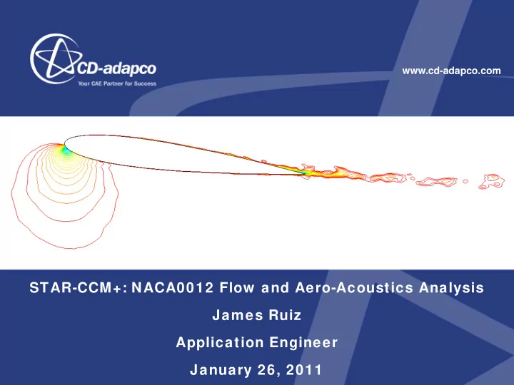
www.cd-adapco.com STAR-CCM+: NACA0012 Flow and Aero-Acoustics Analysis James Ruiz Application Engineer January 26, 2011
Introduction The objective of this work is to prove the capability of STAR-CCM+ as a Computational Fluid Dynamics • (CFD) software in the analysis of airfoil aero-acoustic and far-field noise propagation. This work in this report focuses on the aeroacoustic performance of a NACA0012 series airfoil. • Test conditions for the airfoil are listed on the following slide. • The goal is to determine the peak sound pressure level (SPL) relative to 3 rd octave frequency bands and • the frequency that produces the peak SPL. Frequency range of interest for this analysis is between 1 kHz and 1000 kHz. • The work outlined in this report is based on the following publication: • NASA Reference Publication 1218, July 1989 • Airfoil Self-Noise and Prediction Thomas F. Brooks, D. Stuart Pope and Michael A. Marcolini Documented results for SPL are plotted in • 3 rd octave frequencies bands in figure 52 of the NASA publication. The solid black line represents the experimental results. 2
Experimental Data Test Conditions: • Freestream Mach Number: 0.208 (71.3 m/s) • Freestream Temperature: 300 K • Freestream Reynolds Number: 1.13E6 (at 0.2286 m) • Freestream Viscosity: 1.71E-5 Pa-s • Airfoil Angle of Attack: 7.3 degrees • Airfoil Chord Length: 0.2286 m • Airfoil Span: 0.4572 m • Trailing edge thickness: 0.001c • 3
Airfoil and Computational Domain Airfoil: NACA0012 • Angle of Attack 7.3 degrees • Airfoil Span: 0.1286 m • Freestream Diameter: 2.4 m • Trailing Edge Thickness: 0.001c (2.286E-4 m) • 4
Mesh Continuum (Air) Mesh Models: • Surface Remesher • Trimmer • Prism Layer Mesher • Reference Values: • Thickness of near Wall Prism Layer: 1E-5 m • Base size: 4 mm • Maximum cell size: 1600% • Number of prism layers: 20 • Prism layer thickness: 5 mm • Surface size: • Relative minimum size: 1 mm • Relative target size: 2 mm • Template Growth Rate: • Default growth rate: Slow • Boundary growth rate: Medium • 5
Mesh Volumetric Controls 2 mm mm 1 mm mm 6
Volume Mesh Section Cut: Z=0.05715 m • Prism Layers: 20 • Prism Layer Thickness: 5 mm • Prism Layer Stretching: 1.28 • Predominantly hexahedral cells in the free stream domain. • 1 mm mm 0.0312 3125 5 mm 7
Steady State Physics Physics Models: • Air • Three Dimensional • Steady State • Ideal Gas • Segregated Flow Solver • Segregated Energy Solver • K-Omega SST Turbulence • All Y+ wall Treatment • Aeroacoustics • Broadband Noise Sources • Lilley Sources • Reference Values: • Reference pressure: 101325 Pa • Initial Conditions: • Static Pressure: 0.0 Pa (gage) • Static Temperature: 300K • Turbulence Intensity: 0.01 • Turbulent Viscosity Ratio: 10 • 8 Velocity: [ 71.3 , 0 , 0 ] m/s •
Boundary Conditions Boundary Conditions: • Free Stream: • Mach Number: 0.208 • Static Temperature: 300 K • Turbulence Intensity: 0.01 • Turbulent Viscosity Ratio: 10 • 9
Steady State Lift and Drag Coefficients Force coefficients: • Published: • Lift Coefficient: 0.800 • Drag Coefficient: 0.0113 • Simulation: • Lift Coefficient: 0.792 • Drag Coefficient: 0.0180 • Reference values: • Area: 2.965557E-2 m 2 • Velocity: 713 m/s • Density: 1.17683 kg/m 3 • 10
Steady State Mesh Cutoff Frequency Mesh Cutoff Frequency measures the mesh’s ability to capture a given frequency: • Formulation is based on turbulent kinetic energy and cell volume. 2 • k 3 F MC = This tells us that the mesh is red is capable of capturing 1000 Hz. ( Hz ) • 3 2 * V ISO surface shown is MCF = 1000 Hz. • 11
Unsteady LES Physics Air: • Three Dimensional • Implicit Unsteady • Discretization: 2 nd Order • Ideal Gas • Segregated Flow Solver • Convection: Bounded-Central • Segregated Energy Solver • LES Turbulence • Wale Subgrid Scale Model • All Y+ Wall Treatment • Aeroacoustics • Ffwocs Williams-Hawkings • Reference Values: • Reference pressure: 101325 Pa • Initial Conditions: • Started from Steady State RANS calculation. • 12
Time Step and Duration Calculate the time step based the highest frequency to be resolved: 1 = [ ] TimeStep s 10 * MaximumFre quenc Re solution [ Hz ] Highest frequency to be resolved: 10,000 Hz • Time step: 1E-5 s • Calculate the duration based the minimum frequency to be resolved: 20 = Duration [ s ] MinimumFre quency Re solution [ Hz ] Minimum frequency to be resolved: 1,000 Hz • Duration: 0.02 s • 13
Unsteady LES Lift and Drag Coefficients Force coefficients: • Published: • Lift Coefficient: 0.800 • Drag Coefficient: 0.0113 • Simulation: • Lift Coefficient: 0.8428 • Drag Coefficient: 0.0122 • Reference values: • Area: 2.965557E-2 m 2 • Velocity: 713 m/s • Density: 1.17683 kg/m 3 • Viewing the lift and drag coefficients on • a per iteration basis allows us to ensure convergence within the time step. 15 inner iterations are used to achieve • convergence within the time step. 14
Scalar Contours 15
Pressure Probes Pressure probes around the airfoil surface at mid-span track pressure fluctuations as a function of time. • Pressure probes are numbered 1-18 from the leading edge of the airfoil past the trialing edge of the airfoil. • Tracking pressure allows us todetermine when the • pressure fluctuations become stable. Viewing the pressure fluctuations on a per iteration • basis allows us to ensure convergence within the time step. Only 8-10 inner iterations are required achieve • convergence within the time step. This is less restrictive than the force convergence requirement. 16
FWH Receivers Receiver locations listed in NASA publication: • M1: [ 0.2286 , 1.22 , 0.05715 ] m • M2: [ 0.2286 , -1.22 , 0.05715 ] m • M4: [ -0.3814 , 1.05655 , 0.05715 ] m • M5: [ 0.8386 , 1.05655 , 0.05715 ] m • M7: [ -0.3814 , -1.05655 , 0.05715 ] m • M8: [ 0.8386 , -1.05655 , 0.05715 ] m • For the sake of acoustic analysis, a single observer point located • at receiver point M1 is used for spectra analysis. The time it takes the pressure fluctuations to • propagate from the FWH surface to the FWH receiver depends on speed of sound of the surrounding media and distance between the surfaces and receivers. Dis tan ce [ m ] 1 . 22 = = = Time [ s ] 0 . 00359 [ s ] SpeedofSou nd [ m / s ] 340 Sufficient duration of the analysis is required to wash • out any transient effects in the receiver data and must also be sufficient to capture 0.02 s of statistically stable data. 17
Sound Pressure Level (LES) Receiver data processed using a Fourier Transform of sound pressure level versus 3 rd octave frequency • bands. A factor must be added to the overall SPL to account for the variation in span from the experimental airfoil to • the analysis airfoil: L 0 . 4572 = = = Experiment SPL [ dB ] 10 log 10 log 5 . 5 [ dB ] 10 10 L 0 . 1286 Analysis Simulation Peak SPL: 65.5 dB • Exact center frequency: 1589.9 Hz • Experiment Peak SPL: 67 dB • Exact center frequency: 1258.9 Hz • 18
Setup & Run Statistics (LES Analysis) Compute Resources: • Processor: Intel Xeon • RAM per processor: 2 Gb • Number of processors: 40 • Processor Speed: 2.6 Ghz • Number of compute cells: 9.5 M • Operating System: LINUX 64-bit • Total run time: • Simulated Time: 0.04 s • Wall Clock Time: 89 hrs (3.7 days) • Wall Clock Time per Iteration: 5.34 s • Wall Clock Time per Time Step: 80.1 s (15 inner iterations) • 19
Conclusion CAD CA Regi egion Sur urfa face Volum ume Physi ysics cs Pos ost t Solv lve Creati eation Setu etup Mes esh Mes esh Proce cess ss Setu etup Man hrs: 1.0 Man hrs: 0.5 Man hrs: 1.0 Cell count: 9.5M Man hrs: 0.5 Man hrs: 1.0 Inner Iterations: 15 CPU hrs: 0.5 Time Steps: 4000 Physical Time: 0.04 s CPU hrs: 89 (3.7 days) Sound Pressure Level Results (1000 – 10000 Hz frequency range): • Experiment Peak SPL: 67 dB • Simulation Peak SPL: 65.5 dB (2% difference) • Peak frequency: 1589.9 Hz (1 band difference) • Setup and simulation time for LES anaoysis: 4 days • 20
Sound Pressure Level (Unsteady RANS) A similar acoustic analysis was performed using a unsteady RANS turbulence model (K-Omega SST). • The objective was to determine if using a URANS based turbulence model will predict the correct frequency at • which the peak sound pressure level is achieved. In a similar manner, the receiver data is processed • using a Fourier Transform to obtain a sound pressure level versus 3 rd octave band frequencies. The SPL was then adjusted to account for the • span of the experimental airfoil. Simulation Peak SPL: 60.5 dB • Exact center frequency: 1258.9 Hz • Experiment Peak SPL: 67 dB • Exact center frequency: 1258.9 Hz • 21
Recommend
More recommend
Unleash a World of Digital Possibilities—Browse, Share, and Explore Content Without Boundaries