Data-flow analysis Introduction to data-flow analysis Michel - PDF document

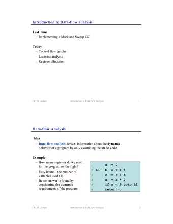
Data-flow analysis Introduction to data-flow analysis Michel Schinz – based on material by Erik Stenman and Michael Schwartzbach Data-flow analysis Example: liveness Data-flow analysis is a global analysis framework that can be used to compute – or, more precisely, approximate – various properties of programs. A variable is said to be live at a given point if its value will be read later. While liveness is clearly undecidable, a The results of those analysis can be used to perform several conservative approximation can be computed using data- optimisations, for example: flow analysis. • common sub-expression elimination, This approximation can then be used, for example, to • dead-code elimination, allocate registers: a set of variables that are never live at the • constant propagation, same time can share a single register. • register allocation, • etc. 3 4 Requirements Data-flow analysis requires the program to be represented as a control flow graph (CFG). Control-flow graphs To compute properties about the program, it assigns values to the nodes of the CFG. Those values must be related to each other by a special kind of partial order called a lattice. We therefore start by introducing control flow graphs and lattice theory. 5

Control-flow graph CFG example x � 12 A control flow graph ( CFG ) is a graphical representation of a program. y � 5 The nodes of the CFG are the statements of that program. The edges of the CFG represent the flow of control: there is if x<y an edge from n 1 to n 2 if and only if control can flow immediately from n 1 to n 2 . That is, if the statements of n 1 and n 2 can be executed in direct succession. x � y x � 2*y z � x/y 7 8 Predecessors and successors Basic block A basic block is a maximal sequence of statements for which control flow is purely linear. In the CFG, the set of the immediate predecessors of a node That is, control always enters a basic block from the top – n is written pred( n ). its first instruction – and leaves from the bottom – its last Similarly, the set of the immediate successors of a node n is instruction. written succ( n ). Basic blocks are often used as the nodes of a CFG, in order to reduce its size. 9 10 CFG example (basic blocks) x � 12 y � 5 if x<y Lattice theory x � y x � 2*y z � x/y 11

Partial order Partial order example A partial order is a mathematical structure ( S , � )composed In Java, the set of types along with the subtyping relation of a set S and a binary relation � on S , satisfying the form a partial order. following conditions: According to that order, the type String is smaller ( i.e. a 1. reflexivity: ∀ x ∈ S , x � x subtype) of the type Object . 2. transitivity: ∀ x , y , z ∈ S , x � y � y � z ⇒ x � z The type String and Integer are not comparable: none of them is a subtype of the other. 3. anti-symmetry: ∀ x , y ∈ S , x � y � y � x ⇒ x = y 13 14 Upper bound Lower bound Given a partial order ( S , � ) and a set X ⊆ S , y ∈ S is an Given a partial order ( S , � ) and a set X ⊆ S , y ∈ S is a lower upper bound for X , written X � y , if bound for X , written y � X , if ∀ x ∈ X , x � y . ∀ x ∈ X , y � x . A least upper bound ( lub ) for X , written � X , is defined by: A greatest lower bound for X , written � X , is defined by: X � � X � ∀ y ∈ S , X � y ⇒ � X � y � X � X � ∀ y ∈ S , y � X ⇒ y � � X Notice that a least upper bound does not always exist. Notice that a greatest lower bound does not always exist. 15 16 Lattice Finite partial orders A lattice is a partial order L = ( S , � ) for which � X and � X A partial order ( S , � ) is finite if the set S contains a finite exist for all X ⊆ S . number of elements. A lattice has a unique greatest element, written ! and For such partial orders, the lattice requirements reduce to pronounced “ top ”, defined as ! = � S . the following: It also has a unique smallest element, written ⊥ and • ! and ⊥ exist, pronounced “ bottom ”, defined as ⊥ = � S . • every pair of elements x , y in S has a least upper bound – written x � y – as well as a greatest lower bound – The height of a lattice is the length of the longest path from written x � y . ⊥ to ! . 17 18

Cover relation Hasse diagram A partial order can be represented graphically by a Hasse In a partial order ( S , � ), we say that an element y covers diagram . another element x if: In such a diagram, the elements of the set are represented ( x � y ) ∧ ( ∀ z ∈ S , x � z � y ⇒ x = z ) by dots. where x � y ⇔ x � y ∧ x � y . If an element y covers an element x , then the dot of y is Intuitively, y covers x if y is the smallest element greater placed above the dot of x , and a line is drawn to connect than x . the two dots. 19 20 Hasse diagram example Partial order examples Which of the following partial orders are lattices? Hasse diagram for the partial order ( S , � ) where S = { 0, 1, …, 7 } and x � y ⇔ ( x & y ) = x 1 2 3 bitwise and 7 (111) 3 (011) 6 (110) 5 (101) 4 5 6 2 (010) 1 (001) 4 (100) 0 (000) 21 22 Monotone function A function f : L � L is monotone if and only if: ∀ x , y ∈ S , x � y ⇒ f ( x ) � f ( y ) Fixed points This does not imply that f is increasing, as constant functions are also monotone. Viewed as functions, � and � are monotone in both arguments. 24

⊆ Fixed point theorem Fixed points and equations Fixed points are interesting as they enable us to solve systems of equations of the following form: x 1 = F 1 ( x 1 , …, x n ) Definition: a value v is a fixed point of a function f if and x 2 = F 2 ( x 1 , …, x n ) only if f ( v ) = v . … Fixed point theorem: In a lattice L with finite height, every x n = F n ( x 1 , …, x n ) monotone function f has a unique least fixed point fix( f ), where x 1 , ..., x n are variables, and F 1 , ..., F n : L n � L are and it is given by: monotone functions. fix( f ) = ⊥ � f ( ⊥ ) � f 2 ( ⊥ ) � f 3 ( ⊥ ) � … Such a system has a unique least solution that is the least fixed point of the composite function F : L n � L n defined as: F ( x 1 , …, x n ) = ( F 1 ( x 1 , …, x n ), …, F n ( x 1 , …, x n ) ) 25 26 Fixed points and inequations Systems of inequations of the following form: x 1 � F 1 ( x 1 , …, x n ) x 2 � F 2 ( x 1 , …, x n ) Data-flow analysis … x n � F n ( x 1 , …, x n ) can be solved similarly by observing that x � y ⇔ x = x � y and rewriting the inequations. 27 Overview Example: liveness Data-flow analysis works on a control-flow graph and a lattice L . The lattice can either be fixed for all programs, or As we have seen, liveness is a property that can be depend on the analysed one. approximated using data-flow analysis. A variable v n ranging over the values of L is attached to The lattice to use in that case is L = { P (V), } where V is every node n of the CFG. the set of variables appearing in the analysed program, and A set of (in)equations for these variables are then extracted P is the power set operator (set of all subsets). from the CFG – according to the analysis being performed – and solved using the fixed point technique. 29 30

Example: liveness Example: liveness For a program containing three variables x , y and z , the lattice for liveness is the following: To every node n in the CFG, we attach a variable v n giving { x , y , z } the set of variables live before that node. The value of that variable is given by: v n = ( v s1 � v s2 � … \ written( n )) � read( n ) { x , y } { x , z } { y , z } where s 1 , s 2 , … are the successors of n , read( n ) is the set of program variables read by n , and written( n ) is the set of { x } { y } { z } variables written by n . {} 31 32 Example: liveness Fixed point algorithm To solve the data-flow constraints, we construct the composite function F and compute its least fixed point by CFG constraints solution iteration. 1 x � read-int F ( x 1 , x 2 , x 3 , x 4 , x 5 , x 6 ) = ( x 2 \{ x }, x 3 \{ y }, x 4 � x 5 � { x , y }, x 6 � { x }\{ z }, x 6 � { y }\{ z }, { z }) v 1 = v 2 \ { x } v 1 = { } 2 y � read-int v 2 = v 3 \ { y } v 2 = { x } v 3 = v 4 ∪ v 5 ∪ { x , y } v 3 = { x , y } Iteration x 1 x 2 x 3 x 4 x 5 x 6 3 if (x < y) v 4 = v 6 ∪ { x } \ { z } v 4 = { x } 0 { � } { � } { � } { � } { � } { � } v 5 = v 6 ∪ { y } \ { z } v 5 = { y } 1 { } { } { x , y } { x } { y } { z } 4 z � x 5 z � y v 6 = { z } v 6 = { z } 2 { } { x � } { x , y } { x } { y } { z } 3 { } { x � } { x , y } { x } { y } { z } 6 print-int z 33 34 Work-list algorithm Work-list algorithm x 1 = x 2 = … = x n = ⊥ Computing the fixed point by simple iteration as we did q = [ v 1 , …, v n ] works, but is wasteful as the information for all nodes is re- while ( q � []) computed at every iteration. assume q = [ v i , … ] It is possible to do better by remembering, for every y = F i ( x 1 , …, x n ) variable v , the set dep( v ) of the variables whose value q = q .tail depends on the value of v itself. if ( y � x i ) Then, whenever the value of some variable v changes, we for ( v ∈ dep( v i )) only re-compute the value of the variables that belong to if ( v ∉ q ) q .append( v ) dep( v ). x i = y 35 36