Stability Prof. Seungchul Lee Industrial AI Lab. Most Slides from - PowerPoint PPT Presentation
Stability Prof. Seungchul Lee Industrial AI Lab. Most Slides from the Routh-Hurwitz Criterion by Brian Douglas and Control by Prof. Richard Hill Stability of Open Loop System () In order for a system = () to be
Stability Prof. Seungchul Lee Industrial AI Lab. Most Slides from the Routh-Hurwitz Criterion by Brian Douglas and Control by Prof. Richard Hill
Stability of Open Loop System 𝑂(𝑡) • In order for a system 𝐻 𝑡 = 𝐸(𝑡) to be stable all of the roots of the characteristic polynomial need to lie in the left-half plane (LHP). – The characteristic equation is the denominator of the transfer function. – The roots of the characteristic equation are the exact same as the poles of the transfer function. – The eigenvalues of matrix 𝐵 in the equivalent state space representation are the same as the roots of the characteristic polynomial. – In order to have a stable system, roots of 𝐻(𝑡) must be in LHP. 2
Stability of Open Loop System • When a pole is negative – This root exists in the left half plane – Transfer function will ultimately die out – The system will eventually be at rest (stable) • When a pole is positive – This root exists in the right half plane – Transfer function will blow up into infinity – The system is unstable • Transfer function of multiple poles – The last one blows up to infinity to make the whole transfer function unstable – Conclusion: a single root in the right half plane makes the whole system unstable 3
Routh-Hurwitz Criterion 4
Routh-Hurwitz Criterion • Calculating the roots of the system for larger than the second-order polynomial becomes time- consuming and possibly even impossible in a closed-form • How can we determine the stability of a higher order polynomial without solving for the roots directly? – The great thing about the Routh-Hurwitz criterion is that you do not have to solve for the roots of the characteristic equation – If all of the signs are not the same, the system is unstable – If you build up a transfer function with a series of poles, then the only way to get a negative coefficient is to have at least one pole exists in right-half plane 5
Routh-Hurwitz Criterion • However, we cannot claim that all positive coefficients are still either stable or unstable 6
Normal Case (1/2) • Routh array is a table that can be populated with the coefficients of the polynomial with a few simple rules – The number of RHP roots of 𝐸(𝑡) is equal to the number of sign changes in the left column of the Routh array 7
Normal Case (2/2) • Determine the number of roots in RHP by counting the number of sign changes – We can determine the number of roots in the right-half plane by looking at this first column – It changes sign twice which means that there are two roots in the right half plane 8
Special Case 1 (1/2) • A zero in a row with at least one non-zero appearing later in that same row – If you are attempting to access stability of the system, you do not need to complete the rest of the table at this point – The system is always unstable because completing Routh array will always result in a sign change of the first column 9
Special Case 1 (2/2) • If you are interested in the number of roots located in the right half plane, you can complete the table like below – You replace that zero with the Greek symbol epsilon 𝜗 > 0 – When you finish completing the table, you can take the limit as epsilon 𝜗 goes to zero – You can see that we still have two unstable roots or two roots in the right half plane 10
Special Case 2 (1/2) • The second special case is when there is an entire row of zeros, not just a single zero in the row • Auxiliary polynomial 𝑄(𝑡) : the row directly above the row of zeros 11
Special Case 2 (2/2) • Then 𝑄(𝑡) is a factor of the original polynomial 𝐸(𝑡) • Apply the Routh-Hurwitz criterion again to 𝑆(𝑡) 12
Stability with State Space Representation 13
Stability with State Space Representation • It is useful to start with scalar systems to get some intuition about what is going on • From scalars to matrices? • We cannot say that 𝐵 > 0 , but we can do the next best thing - eigenvalues ! 14
Stability with State Space Representation • The eigenvalues tell us how the matrix 𝐵 ‘acts’ in different directions (eigenvectors) 15
Stability of Closed Loop System 16
Root Locus (Stability in Time) • We are interested in the stability of a closed loop system from an open loop system. • The closed-loop system is • A pole exists when the characteristic polynomial in the denominator becomes zero. 17
Root Locus (Stability in Time) • A value of 𝑡 ∗ is a closed loop pole if • Closed-loop poles in the LHP indicate stability – The closeness of the poles to the RHP indicate how near to instability the system is 18
Relative Stability (Stability in Frequency) • Suppose the Bode plot of the open-loop transfer function is given. • Question: – tell the stability of a closed-loop system from the open-loop frequency response 19
Relative Stability (Stability in Frequency) • At 180 o of phase lag of the loop, the reference and feedback signal are added. – If the magnitude of the loop is greater than 1 the error grows exponentially (unstable) 20
Relative Stability • Relative stability is indicated by how close the open-loop frequency response is to the point of 180 o of phase lag and a magnitude of 1 • More specifically, – Gain margin is the distance from a magnitude of 1 (0 dB) at the frequency where 𝜚 = 180 𝑝 (phase crossover frequency) – Phase margin is the distance from a phase of -180 o at the frequency where M = 0 dB (gain crossover frequency) 21
Relative Stability • In order to be stable, both gain and phase margin must be positive • Gain and phase margins tell how stable the system would be in closed-loop – These quantities can be read from the open-loop data 22
Relative Stability (Stability in Frequency) • What if 𝐿 proportional controller is implemented? • More intuitively, – Gain margin indicates how much you can increase the loop gain 𝐿 before the system goes unstable – Phase margin indicates the amount of phase lag (time delay) you can add before the system goes unstable 23
Relative Stability in MATLAB 24
Relative Stability in MATLAB • Is stable the closed-loop system with a unity negative feedback? 25
Gain Margin 26
Gain Margin 27
Phase Margin • Add more delay 28
Phase Margin 29
Phase Margin 30
Stability in Nyquist Plot 31
Stability in Nyquist Plot 1 𝐻(𝑘𝜕) when ∠𝐻 𝑘𝜕 = 180 𝑝 • The gain margin, 𝐿 𝑛 = – 𝐿 𝑛 is the maximum stable gain in closed loop – It is easy to find the maximum stable gain from the Nyquist plot • The phase margin, Φ 𝑛 is the uniform phase change required to destabilize the system under unitary feedback 32
Stability in Nyquist Plot • What if 𝐿 proportional controller is implemented? – Gain margin indicates how much you can increase the loop gain 𝐿 before the system goes unstable – Phase margin indicates the amount of phase lag (time delay) you can add before the system goes unstable 33
Nyquist Stability in MATLAB 34
Nyquist Stability in MATLAB 35
Nyquist Stability in MATLAB 36
Nyquist Stability in MATLAB 37
Nyquist Stability in MATLAB 38
Recommend
More recommend
Explore More Topics
Stay informed with curated content and fresh updates.


