SQUAREM Acceleration Schemes for Monotone Fixed-Point Iterations - PowerPoint PPT Presentation
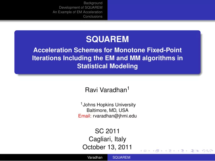
Background Development of SQUAREM An Example of EM Acceleration Conclusions SQUAREM Acceleration Schemes for Monotone Fixed-Point Iterations Including the EM and MM algorithms in Statistical Modeling Ravi Varadhan 1 1 Johns Hopkins University
Background Development of SQUAREM An Example of EM Acceleration Conclusions SQUAREM Acceleration Schemes for Monotone Fixed-Point Iterations Including the EM and MM algorithms in Statistical Modeling Ravi Varadhan 1 1 Johns Hopkins University Baltimore, MD, USA Email: rvaradhan@jhmi.edu SC 2011 Cagliari, Italy October 13, 2011 Varadhan SQUAREM
Background Development of SQUAREM Fixed-Point Iterations An Example of EM Acceleration EM and MM Conclusions Gratitude Professor Claude Brezinski Christophe Roland Marcos Raydan R Core Development Team Varadhan SQUAREM
Background Development of SQUAREM Fixed-Point Iterations An Example of EM Acceleration EM and MM Conclusions Fixed-Point Iteration x k + 1 = F ( x k ) , k = 0 , 1 , . . . . F : Ω ⊂ R p �→ Ω , and differentiable F is a contraction: || F ( x ) − F ( y ) || ≤ || x − y || , ∀ x , y ∈ Ω Associated Lyapunov function L ( x ) such that L ( x k + 1 ) ≥ L ( x k ) Guaranteed convergence: { x k } → x ∗ ∈ Ω Varadhan SQUAREM
Background Development of SQUAREM Fixed-Point Iterations An Example of EM Acceleration EM and MM Conclusions EM Algorithm Let y , z , x , be observed, missing, and complete data, respectively. The k -th step of the iteration: θ k + 1 = argmax Q ( θ | θ k ); k = 0 , 1 , . . . , where Q ( θ | θ k ) = E [ L c ( θ ) | y , θ k ] , � = L c ( θ ) f ( z | y , θ k ) dz , Ascent property: L obs ( θ k + 1 ) ≥ L obs ( θ k ) The goal is to maximize L obs ( θ ; y ) Varadhan SQUAREM
Background Development of SQUAREM Fixed-Point Iterations An Example of EM Acceleration EM and MM Conclusions Why is EM So Popular? Seminal work of Dempster, Laird, and Rubin (1977) Most popular approach in computational statistics Computes MLE in “incomplete” data type problems Reduces incomplete-data problem (difficult) to complete-data problem (easier). Versatile, stable (ascent property), globally convergent under weak regularity conditions (Wu, 1983) Meng’s paper: EM: An old folk song sung to a new tune Varadhan SQUAREM
Background Development of SQUAREM Fixed-Point Iterations An Example of EM Acceleration EM and MM Conclusions MM Algorithm A majorizing function, g ( θ | θ k ) : f ( θ k ) = g ( θ k | θ k ) , f ( θ ) ≤ g ( θ | θ k ) , ∀ θ. To minimize f ( θ ) , construct a majorizing function and minimize it (MM) θ k + 1 = argmin g ( θ | θ k ); k = 0 , 1 , . . . Descent property: f ( θ k + 1 ) ≤ f ( θ k ) EM may be viewed as a subclass of MM. Varadhan SQUAREM
Background Development of SQUAREM Fixed-Point Iterations An Example of EM Acceleration EM and MM Conclusions Linear Convergence of EM/MM The EM/MM as a fixed-point iteration F : θ k + 1 = F ( θ k ) , k = 0 , 1 , . . . . Assume θ k → θ ∗ and F is differentiable at θ ∗ , θ k + 1 − θ ∗ = J ( θ ∗ )( θ k − θ ∗ ) + o ( � θ k − θ ∗ � 2 ) , Jacobian of F can be written as (DLR77): J ( θ ∗ ) I miss ( θ ∗ ; y ) I − 1 comp ( θ ∗ ; y ) = I p × p − I obs ( θ ∗ ; y ) I − 1 comp ( θ ∗ ; y ) = Rate of convergence ∝ ρ [ J ( θ ∗ )] . Varadhan SQUAREM
Background Development of SQUAREM Fixed-Point Iterations An Example of EM Acceleration EM and MM Conclusions Why Accelerate the EM? Slow, linear convergence in practice. Acceleration is useful in: high-dimensional and/or large scale problems (e.g., PET imaging, machine learning) complex statistical models (e.g., GLMM, NLME, longitudinal data) repeated model estimation (e.g., simulations, bootstrapping) Varadhan SQUAREM
Background Development of SQUAREM Fixed-Point Iterations An Example of EM Acceleration EM and MM Conclusions What is Desirable in an Accelerator? Ken Lange (1995) - “it is likely that no acceleration method can match the stability and simplicity of the unadorned EM algorithm.” Simple and easy to apply (low intellectual and implementation costs) Stability (monotonicity and/or global convergence) Generally applicable to (most) all EM problems (exception, MCEM) Automatic - no problem-specific “tweaking”. Without much additional information (e.g., gradient/hessian of L obs ) Varadhan SQUAREM
Background Development of SQUAREM An Example of EM Acceleration Conclusions Iterative Acceleration Schemes At least 2 ways to motivate these acceleration methods Vector sequence extrapolation with cycling 1 Classical Newton-type root-finders 2 Varadhan SQUAREM
Background Development of SQUAREM An Example of EM Acceleration Conclusions Steffensen-Type Methods (STEM) Define g ( θ ) = F ( θ ) − θ ; M n = J ( θ n ) − I ; u 0 = θ n ; u 1 = F ( θ n ); r n = u 1 − u 0 ; v n = g ( u 1 ) − g ( u 0 ) Newton’s method is obtained by finding the zero of the linear approximation of g ( θ ) : g ( θ ) = g ( u 0 ) + M n . ( θ − u 0 ) . 1 α n I , and write two We approximate M n with the scalar matrix different approximations for the fixed point θ ∗ : g ( θ ∗ ) = 0: t 0 = u 0 − α n g ( u 0 ) n + 1 t 1 = u 1 − α n g ( u 1 ) . n + 1 Varadhan SQUAREM
Background Development of SQUAREM An Example of EM Acceleration Conclusions Steffensen-Type Methods(STEM) We now choose α n to minimize discrepancy between t 0 n + 1 and t 1 n + 1 . An obvious measure of discrepancy is � t 1 n + 1 − t 0 n + 1 � 2 , yielding steplength α n = r T n v n , (1) v T n v n Another measure of discrepancy: � t 1 n + 1 − t 0 n + 1 � 2 /α 2 n , yielding the steplength α n = r T n r n . (2) r T n v n Another minimizes the discrepancy: −� t 1 n + 1 − t 0 n + 1 � 2 /α n , where α n < 0: α n = − � r n � � v n � . (3) Varadhan SQUAREM
Background Development of SQUAREM An Example of EM Acceleration Conclusions STEM STEM: θ n + 1 = θ n − α n r n , where r n = F ( θ n ) − θ n and v n = F ( F ( θ n )) − 2 F ( θ n ) + θ n . α n can be one of 3 steplengths as defined in previous slide. Mediocre performance. How can we improve it? Varadhan SQUAREM
Background Development of SQUAREM An Example of EM Acceleration Conclusions Cauchy-Barzilai-Borwein Motivation: Cauchy-Barzilai-Borwein for quadratic minimization (Raydan and Svaiter, 2002) min f ( x ) = 1 2 x T Ax + b T x where A is symmetric and positive-definite. Cauchy (steepest-descent) ill-conditioned when ρ ( A ) ≈ 1 Barzilai-Borwein gradient method uses previous steplength RS2002 combined Cauchy and BB to obtain: x n + 1 = x n − 2 α n g n + α 2 n h n where g n = Ax n − b n , h n = Ag n , α n = g T n g n g T n h n Varadhan SQUAREM
Background Development of SQUAREM An Example of EM Acceleration Conclusions SQUAREM SQUAREM: θ n + 1 = θ n − 2 α n r n + α 2 n v n . SqS1: α n = r T n v n v T n v n SqS2: α n = r T n r n r T n v n SqS3: α n = − � r n � � v n � , Varadhan SQUAREM
Background Development of SQUAREM An Example of EM Acceleration Conclusions Pseudocode of SQUAREM While not converged 1. θ 1 = F ( θ 0 ) 2. θ 2 = F ( θ 1 ) 3. r = θ 1 − θ 0 4. v = ( θ 2 − θ 1 ) − r 5. Compute α with r and v . θ ′ = θ 0 − 2 α r + α 2 v 6. θ 0 = F ( θ ′ ) (stabilization) 7. 8. Check for convergence. Varadhan SQUAREM
Background Development of SQUAREM An Example of EM Acceleration Conclusions SQUAREM An R package implementing a family of algorithms for speeding-up any slowly convergent multivariate sequence from a monotone fixed-point mapping Also contains higher-order cycled, squared, extrapolation schemes Very easy to use Ideal for high-dimensional problems Input: fixptfn = fixed-point mapping F Optional Input: objfn = merit function (if any) Two main control parameter choices: order of extrapolation and monotonicity Available on CRAN . Varadhan SQUAREM
Background Development of SQUAREM An Example of EM Acceleration Conclusions Table: Data from The London Times on deaths during 1910-1912 Deaths, y i Frequency, n i Deaths, y i Frequency, n i 0 162 5 61 1 267 6 27 2 271 7 8 3 185 8 3 4 111 9 1 Varadhan SQUAREM
Background Development of SQUAREM An Example of EM Acceleration Conclusions Binary Poisson Mixture The incomplete-data likelihood: 9 � n i . � � pe − µ 1 µ i 1 / i ! + ( 1 − p ) e − µ 2 µ i 2 / i ! i = 0 The EM algorithm is as follows: p ( k + 1 ) = π ( k ) � � � n i ˆ n i , i 1 i i µ ( k + 1 ) π ( k ) π ( k ) � � � = i n i ˆ n i ˆ ij , j = 1 , 2 , j ij i i 2 � i � i e − µ ( k ) e − µ ( k ) = p ( k ) � � π ( k ) µ ( k ) p ( k ) µ ( k ) j / � l , j = 1 , 2 . ˆ ij j l l l = 1 Varadhan SQUAREM
Background Development of SQUAREM An Example of EM Acceleration Conclusions Binary Poisson Mixture (cont...) MLE: ( p , µ 1 , µ 2 ) = ( 0 . 3599 , 1 . 256 , 2 . 663 ) . Eigenvalues of Jacobian at MLE: (0.9957, 0.7204 and 0) Eigenvalues of ( J − I ) − 1 : (-1, -3.58, and -230.7) Major separation of the largest eigenvalue. Steplength α n must approximate all eigenvalues. EM always takes α n = − 1 . Varadhan SQUAREM
Background Development of SQUAREM An Example of EM Acceleration Conclusions Performance of Schemes Table: Poisson mixture estimation: initial guess θ 0 = (0.3, 1.0, 2.5) EM S1 S2 S3 SqS1 SqS2 SqS3 CPU (sec) 0.26 0.11 0.13 0.16 0.01 0.03 0 fevals 2055 396 477 576 66 84 66 log-lik − 1989.9 − 1989.9 − 1989.9 − 1989.9 − 1989.9 − 1989.9 − 1989.9 Varadhan SQUAREM
Recommend
More recommend
Explore More Topics
Stay informed with curated content and fresh updates.
