p(E|H p(E|H p ) p ) p(E|H p(E|H d ) d ) Concerns Logically - PowerPoint PPT Presentation
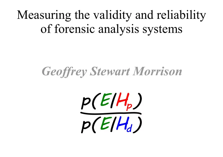
Measuring the validity and reliability of forensic analysis systems Geoffrey Stewart Morrison p(E|H p(E|H p ) p ) p(E|H p(E|H d ) d ) Concerns Logically correct framework for evaluation of forensic evidence - ENFSI Guideline for
Measuring the validity and reliability of forensic analysis systems Geoffrey Stewart Morrison p(E|H p(E|H p ) p ) p(E|H p(E|H d ) d )
Concerns � Logically correct framework for evaluation of forensic evidence - ENFSI Guideline for Evaluative Reporting 2015 � But what is the warrant for the opinion expressed? Where do the numbers come from? - R v T 2010 Risinger at ICFIS 2011 ; � Demonstrate validity and reliability - Daubert 1993; NRC Report 2009; FSR Guidance on validation ; CPD 19A 2015; PCAST Report 2016 2014 � Transparency - R v T 2010 � Reduce potential for cognitive bias - NIST/NIJ Fingerprint nalysis 2012 a ; NCFS task-relevant information 2015 � Communicate strength of forensic evidence to triers of fact
Paradigm � Use of the likelihood-ratio framework for the evaluation of forensic evidence – logically correct � Use of relevant data (data representative of the relevant population), quantitative measurements, and statistical models – transparent and replicable – relatively robust to cognitive bias � Empirical testing of validity and reliability under conditions reflecting those of the case under investigation, using test data drawn from the relevant population – only way to know how well it works
Validity and Reliability (Accuracy and Precision)
not not precise precise not accurate accurate
Measuring Validity
Measuring Validity � Test set consisting of a large number of pairs of samples, some known to have the same origin and some known to have different origins � Test set must represent the relevant population and reflect the conditions of the case at trial � Use forensic-comparison system to calculate LR for each pair � Compare output with knowledge about input
BLACK BOX 156
1 BLACK BOX 78
To be, or not BLACK BOX to be, that is the question
To be, or not to be, that is the question
-3 x 10 1.5 4 Frequency (kHz) 1 3 1024 0.5 2 1 0 1,000,000 1980 0.1 0.2 0.3 0.4 0.5 0.6 0.7 0.8 1990 380 Time (s) 2000 390 400 2010 410 2020 420 2030 430 2040 440 To be, or 42 not to be
BLACK BOX BLACK BOX 1024 1,000,000 To be, or BLACK BOX BLACK BOX 42 not to be
Measuring Validity � Correct-classification / classification-error rate is not appropriate – based on posterior probabilities – hard threshold rather than gradient decision fact same different same correct false acceptance rejection different false correct acceptance rejection
Measuring Validity � Correct-classification / classification-error rate is not appropriate – based on posterior probabilities – hard threshold rather than gradient decision fact same different same miss false different alarm
Measuring Validity � Correct-classification / classification-error rate is not appropriate – based on posterior probabilities – hard threshold rather than gradient decision fact same different same 0 1 1 0 different
miss false alarm 9 8 classification error rate 7 6 5 4 3 2 1 -3 -2 -1 0 1 2 3 Log Posterior Odds 10
Measuring Validity � Goodness is to which LRs from same-origin pairs > 1, and extent LRs from different -origin pairs < 1 � Goodness is to which log(LR)s from same-origin pairs > , 0 extent and log(LR)s from different -origin pairs < 0 LR 1/1000 1/100 1/10 1 10 100 1000 -3 -2 -1 0 +1 +2 +3 log (LR) 10
Measuring Validity � A metric which captures the gradient goodness of a set of likelihood ratios derived from test data is the log-likelihood-ratio cost, C llr � � � � � � N N 1 1 1 1 so do � � � � � � � � � � � C log 1 log 1 LR � � � llr 2 2 do � � 2 N LR N j � � � � so i 1 j 1 so do i Brümmer N, du Preez J (2006). , Application independent evaluation of speaker detection Computer Speech & Language , 20, 230–275. doi:10.1016/j.csl.2005.08.001
9 8 7 6 C llr 5 4 3 2 1 -3 -2 -1 0 1 2 3 Log Likelihood Ratio 10
Measuring Validity � System A : C llr = 0.548 � System B: C llr = 0.101 � System C: C llr = 1.018
Tippett Plots
Tippett Plots 1 0.8 cumulative proportion 0.6 0.4 0.2 0 −6 −4 −2 0 2 4 6 log (LR) 10
Tippett Plots 1 0.8 cumulative proportion 0.6 0.4 0.2 0 −6 −4 −2 0 2 4 6 log (LR) 10
Tippett Plots 1 0.8 cumulative proportion 0.6 0.4 0.2 0 −6 −4 −2 0 2 4 6 log (LR) 10
Tippett Plots � System A : C llr = 0.548 � System B: C llr = 0.101
Measuring Reliability
Sources of imprecision � intrinsic variability at the source level – within-source between-sample variability � variability in the transfer process � variability in the measurement technique � variability in sampling of the relevant population � variability in the estimation of statistical model parameters Morrison, G. S. (2016). Special issue on measuring and reporting the precision of forensic likelihood ratios: Introduction to the debate . Science & Justice . doi:10.1016/j.scijus.2016.05.002
Measuring Reliability � Imagine that in the test set we have three recordings ( , A B C , ) of each speaker � A has the same conditions (speaking style, transmission channel, duration, etc.) as the offender recording � B and C have the same conditions as the suspect recording � Use LRs calculated on A - B and A - C pairs to estimate a 95% credible interval (CI)
Measuring Reliability � Two pairs for each same-speaker comparison suspect recording offender recording 001 B 001 A 001 C 001 A 002 B 002 A 002 C 002 A : : : :
Measuring Reliability � Two pairs for each different-speaker comparison suspect recording offender recording 002 B 001 A 00 2 C 001 A 00 3 B 00 1 A 00 3 C 00 1 A : : : : 00 1 B 00 2 A 00 1 C 00 2 A : : : :
Measuring Reliability log(LR) →
Measuring Reliability mean mean log(LR) →
Measuring Reliability → deviation from mean log(LR) → ←
Measuring Reliability → deviation from mean 2.5% 95% 2.5% ←
Measuring Validity & Reliability � System A : C llr = 0.548 95% CI = 0.498 ± � System B: C llr = 0.101 95% CI = 0.988 ±
Measuring Validity & Reliability mean � System A : C = 0.548 C = 0.5 29 95% CI = 0.498 ± llr llr mean � System B: C = 0.101 C = 0. 071 95% CI = 0.988 ± llr llr
Measuring Validity & Reliability 1 1 0.9 0.9 0.8 0.8 0.7 0.7 0.6 0.6 C llr −pooled System A C llr −mean 0.5 0.5 0.4 0.4 0.3 0.3 0.2 0.2 System B 0.1 0.1 0 0 0 0.2 0.4 0.6 0.8 1 credible interval (± orders of magnitude )
Tippett Plots 1 1 0.9 0.9 0.8 0.8 Cumulative Proportion 0.7 Cumulative Proportion 0.7 0.6 0.6 0.5 0.5 0.4 0.4 0.3 0.3 0.2 0.2 0.1 0.1 0 0 −4 −3 −2 −1 0 1 2 3 4 −4 −3 −2 −1 0 1 2 3 4 Log10 Likelihood Ratio Log10 Likelihood Ratio
Summation If the background and test data were consistent with the conditions in a case at trial , and the comparison of the known- and questioned-voice samples resulted in a likelihood ratio of, 00 1 (log 10 LR ( ) of +2 ), and the 95% CI estimate was ±1 orders of magnitude (±1 in log 10 ( LR ) ), then the forensic scientist could make a statementof thefollowingsort:
Based on my evaluation of the evidence, I have calculated that one would be 100 times more likely to obtain the acoustic properties of the questioned-voice sample had been produced by the accused than had it been produced by some other speaker selected at randomfromthepopulation.
What this means is that whatever you believed about the relative probability of the same-speaker hypothesis versus the different- speaker hypothesis before this evidence was presented, you should now believe that the probability of the same-speaker hypothesis relative to the different-speaker hypothesis is 100greaterthanyoubelievedittobebefore.
Based on my calculations, I am 95% certain that the acoustic differences are at least 10 times more likely and not more than 100 times more likely if the questioned-voice sample had been produced by the accused than if it had been produced by someone other than the accused.
Empirical Validation
Empirical Validation � The National Research Council report to Congress on Strengthening Forensic Science in the United States (2009) urged that procedures be adopted which include: � “quantifiable measures of the reliability and accuracy of forensic analyses” (p. 23) � “the reporting of a measurement with an interval that has a high probability of containing the true value” (p. 121) � “the conducting of validation studies of the performance of a forensic procedure” (p. 121)
Recommend
More recommend
Explore More Topics
Stay informed with curated content and fresh updates.


