Spectral Compression of Mesh Geometry Zachi Karni, Craig Gotsman - PowerPoint PPT Presentation

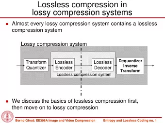
Spectral Compression of Mesh Geometry Zachi Karni, Craig Gotsman SIGGRAPH 2000 1

Introduction ‣ Thus far, topology coding drove geometry coding. ‣ Geometric data contains far more information (15 vs. 3 bits/vertex). ‣ Quantization methods are not suitable for lossy compression. ‣ non-graceful degradation. 2

Intuition 3

Laplace Operator ‣ The Laplace operator is a second order differential operator. ∆ f = f xx + f yy + f zz ‣ One-dimensional heat equation: u t = k ∆ u = ku xx 4

Discrete Laplace Operator ‣ Defined so that the Laplace operator has meaning on a graph or discrete grid (e.g. 3D mesh). ‣ Much discussion over “correct” weights 1 ‣ most commonly: w ij = | i ∗ | 5

Laplacian Smoothing 6

Laplacian Matrix ‣ We can express the discrete Laplacian operator in matrix-vector notation. ∆ x = − Lx, L = I − W ‣ Laplacian matrix in this paper:  i = j 1  L ij = − 1 /d i i and j are neighbors 0 otherwise  7

Spectral Motivation ‣ Regular polygon of n vertices. x 2   x 1 x 3 x 1 x 2   n = 5 :   x = .   . .   x 5 x 4 x 5 ‣ Discrete Laplacian: 8

Spectral Motivation ‣ Discrete Laplacian written in matrix form: 9

Spectral Motivation ‣ n real eigenvalues of K in increasing order: ‣ The n real eigenvectors of K are of the following form: 10

Encoding ‣ Partition the mesh into submeshes. ‣ Compute the topological Laplacian matrix for each little submesh. ‣ Represent each submesh as a linear combination of orthogonal basis functions derived from the eigenvectors of the Laplacian. 11

Decoding ‣ Topology encoded/decoded by your method of choice. ‣ Geometric data sent as coefficient vectors. ‣ Mesh partitioned and eigenvectors computed based on topology, which are then used to decode the geometry. 12

Mesh Signal Processing ‣ Laplacian matrix:  i = j 1  L ij = − 1 /d i i and j are neighbors 0 otherwise  ‣ Eigenvectors form an orthogonal basis of . R n ‣ Associated eigenvalues are the squared frequencies. 13

Mesh Signal Processing Mesh Laplacian Eigen Matrix Eigenvalues 14

Geometry Vectors ‣ We are going to view the geometry as three n-dimensional column vectors (x, y, z), where n is the number of vertices.       x 1 y 1 z 1 x 2 y 2 z 2             x =  y = z = . . .       . . . . . .      x n y n z n 15

Mesh Signal Processing ‣ Since form a basis of n- e 1 , . . . , e n dimensional space, every n-dimensional vector can be written as a linear combination: n x j e j = E ˆ � x = x, ˆ j =1     x 1 x 1 ˆ   | | | x 2 x 2 ˆ      , ˆ e 1 e 2 e n . . . x =  , E = x =     . .  . .     . . | | |    x n x n ˆ 16

Mesh Signal Processing Original model Reconstruction using Reconstruction containing 2,978 100 of the 2,978 basis using 200 basis vertices. functions. functions. 17

Mesh Signal Processing The grayscale intensity of a vertex is proportional to the scalar value of the basis function at that coordinate. Second basis function. Tenth basis function. Hundredth basis function. Eigenvalue = 4.9x10^-4 Eigenvalue = 6.5x10^-2 Eigenvalue = 1.2x10^-1 18

Spectral Coefficient Coding ‣ Uniformly quantize coefficient x , ˆ ˆ y , ˆ z vectors to finite precision (10-16 bits). ‣ Truncate the coefficient vectors. ‣ Encode using Huffman or arithmetic coder. 19

Spectral Coefficient Coding ‣ Trade-off: ‣ Small number of high-precision coefficients ‣ Large number of low-precision coefficients ‣ Optimize based on visual metrics. ‣ Number of retained coefficients per coordinate per submesh chosen such that a visual quality is met. 20

A Visual Metric ‣ RMS geometric distance between corresponding vertices in both models does not capture properties like smoothness. 21

A Visual Metric ‣ Geometric Laplacian: j ∈ n ( i ) l − 1 � ij v j GL ( v i ) = v i − j ∈ n ( i ) l − 1 � ij ‣ Average of the norm of the geometric distance and the norm of the Laplacian distance. � M 1 − M 2 � = 1 � v 1 − v 2 � + � GL ( v 1 ) − GL ( v 2 ) � � � 2 n 22

Mesh Partitioning ‣ Eigenvectors can be calculated in O(n) time since Laplacian is sparse. (n is the number of vertices.) ‣ When n is large, eigenvalues become too close, leading to numerical instability. ‣ Necessary to partition mesh. 23

Mesh Partitioning ‣ Capture local properties better. ‣ Minimize Damage: ‣ roughly same number of vertices in each submesh. ‣ minimize number of edges straddling different submeshes ( edge-cut ). 24

Mesh Partitioning ‣ Optimal solution is NP-Complete. ‣ MeTIS ‣ Optimized linear-time implementation. ‣ Meshes of up to 100,000 vertices. ‣ preference to minimizing the edge-cut over balancing partition. 25

METIS 40 submeshes 70 submeshes 26

Results ‣ Comparison with Touma-Gotsman (TG) compression. 27

Results KG: 3.0 bits/vertex TG: 4.0 bits/vertex KG: 4.1 bits/vertex TG: 4.1 bits/vertex 28

Discussion ‣ Can’t just throw out high frequency detail; it is not noise! ‣ Can’t use the algorithm on very large meshes. MeTIS only accommodates meshes of up to 100,000 vertices. 29