Spectral Clustering Diego Jimnez-Badillo diego_jimenez@inah.gob.mx - PowerPoint PPT Presentation

Analyzing formal features of archaeological artefacts through the application of Spectral Clustering Diego Jiménez-Badillo diego_jimenez@inah.gob.mx National Institute of Anthropology and History México City Salvador Ruíz Correa Omar Méndoza-Montoya src@cimat.mx omendoz@cimat.mx Centro de Investigaciones en Matemáticas Centro de Investigaciones en Matemáticas Guanajuato, Mexico Guanajuato, Mexico

Introduction  This paper is part of a broader effort to introduce the archaeological community to a range of computer tools and mathematical algorithms for analyzing archaeological collections. These include: 1. Application of clustering techniques for unsupervised learning. 2. Acquisition and analysis of 3D digital models. 3. Application of computer vision algorithms for automatic recognition of artefacts. 4. Automatic classification of shape features.

This presentation  Here, we will focus on a new methodology for the analysis of archaeological masks based on a quantitative procedure called Spectral Clustering.  This technique has not been applied before in archaeology despite its proven performance for partitioning a collection of artifacts into meaningful groups.

The Mask Collection from the Great Temple of Tenochtitlan Study case

The idea for this project came from the need to classify similarities in 162 stone masks found in the remains of the Sacred Precinct of Tenochtitlan, the main ceremonial Aztec complex, located in Mexico City. 

The schematic features of these objects set them apart from other more “naturalistic” style artifacts. Their appearance has attracted the attention of many specialists and during the last three decades these masks have been the subject of intense debate for two main reasons:

These masks are interesting for several reasons:  First, 220 figurines and 162 masks were located in 14 Aztec offerings dating from 1390 to 1469 A.C., yet they do not show typical “Aztec features”.

Indeed, their appearance resembles artefacts from Teotihuacan and from the southern State of Guerrero, particularly from the Mezcala region, which is hundreds of kilometers away from the ancient Tenochtitlan.

 Second, it is not clear how many Guerrero/Mezcala styles exist: Some specialists believe there are at least five 1 different traditions while others recognize only four 2 , and another group of researchers sees only two 3 (Serra Puche 1975). 1 Covarrubias 1948, 1961; Olmedo and Gonzalez 1986; Gonzalez and Olmedo 1990 2 Gay, 1967 3 Serra Puche 1975

More objective methods are needed to answer questions such as:  How many styles were developed in the Guerrero/Mezcala regions?  How many of these styles coexisted?  Were some styles contemporary with the Aztecs?  Were some of these masks manufactured by the Aztecs?  Which specific styles are represented among the 162 masks found in the Sacred Precinct of Tenochtitlan?

. Clustering basics

The application of clustering in archaeology One of the most important applications of clustering in archaeology is “ unsupervised learning ”, that is the discovery of artifact groups based exclusively on the analysis of characteristics observed in the artifacts themselves. Once the collection has been segmented into several groups, it would become easier to distinguish potential classes.

Clustering basics Given a set of data-points, any clustering algorithm seeks to separate those points into a finite quantity of groups (i.e., clusters). It applies an objective similarity function to weigh how close (similar) or distant (dissimilar) the original data are among themselves. Items assigned to the same group must be highly similar. At the same time, items belonging to different groups must be highly dissimilar. The quality of the algorithm is judged by how successful it is to accomplish: a) greater homogeneity within a group, and b) greater heterogeneity between groups.

Two clustering approaches are very popular: Component linkage algorithms (i.e. single and total 1. linkage) are based on thresholding pairwise distances and are best suited for discovering complex elongated clusters, but are very sensitive to noise in the data. K-means algorithms, on the other hand, are very 2. robust to noise but are best suited for rounded linearly separable clusters.

Boundary shapes  Some years ago, Olmedo and Gonzalez (1986) proposed a classification based on a component- linkage algorithm (numerical taxonomy).  The forms of faces, eyes, noses, eyebrows, etc. were codified categorically.  This produced an input of 23 shape attributes for each one of 162 masks. Olmedo and Gonzalez. 1986. Presencia del Estilo Mezcala en el Templo Mayor. INAH, México .

Eyebrows shapes Noise shapes

Olmedo and González results  This lead to the identification of 40 groups, of which:  13 groups include only 2 masks  13 groups include only 3 masks  6 groups include 4 masks  20 masks were not included in any group

. Spectral Clustering

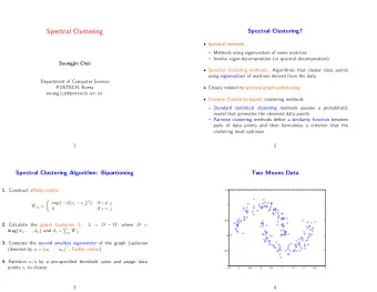
SPECTRAL CLUSTERING Spectral Clustering is a state-of-the-art technique for exploratory analysis. It is derived from Spectral Graph Theory, a branch of mathematics that studies the properties of graphs in relation to the eigenvalues and eigenvectors of an especial type of matrix called Laplacian. In contrast to other techniques, spectral clustering can be applied to different kinds of data, including categorical data. In many situations, categorical data is often the only source of information for archaeological unsupervised learning. Therefore we believe it could bring great benefits in our field.

Here, we won’t dive too deep into mathematical theory. Instead, we follow a very simple example to make the logic of this clustering technique easier to understand. Mathematical proofs can be found in the literature referenced in the paper, especially Luxburg (2007). Spectral Clustering is more efficient than linkage and k- means algorithms. It finds elongated clusters and is more robust to noise than linkage algorithms.

Spectral clustering logic Spectral clustering seeks to identify groups by analyzing no the exact location of the data points (like single, total linkage and k- means), but the connectedness between them.

 Spectral clustering relies on a graph representation of the data set.  In this graph each mask is represented as a vertex. Then, we calculate a measure of similarity (affinity) between all the masks. This is done in two steps:  First, calculate the so-called Hamming distance, which measures the percentage of non-shared attributes between two artefacts. Obviously, this measure is very useful to work with categorical data. The formula is:

 Second, calculate the affinity between all the masks by applying the Gaussian function to the Hamming distance: σ = Threshold to control the desired level of similarity  If two objects are very different the result of the equation is negative and close to or equal to zero. On the contrary, if two objects are very similar the result of the equation is near or equal to 1.

 The next step is to draw a link between two vertices (i.e. masks) if the similarity between them is positive or larger than a certain threshold controlled by the parameter sigma.

Next, we weight each edge of the graph with its corresponding similarity score. This step produces a matrix in which the affinity (i.e. similarity) of all objects with all others is recorded.

 Once this is done, the clustering problem can be reformulated as finding an optimal cutting of the graph. This means finding a partition of the graph such that the edges linking objects of the same group have very high weights (i.e. are quite similar), while the edges between groups have low weighs (i.e. are very dissimilar).

THE CUTTING PROBLEM Finding an optimal cutting of the graph is what mathematicians call an NP-hard problem. This means that it cannot be found in real time. Therefore, we need to find an approximate solution. One type of relaxation is based on analyzing the eigenestructure of the Laplacian matrix associated to the similarity graph. Mathematical proofs can be found in the extensive literature on the subject.

LAPLACIAN MATRIX The so-called Laplacian matrix is a transformation of the similarity matrix that shows more clearly the structure of the dataset. To build a Laplacian Matrix we need two ingredients: A matrix D containing information of the connectivity a. of the similarity graph. This is called the Degree matrix or Diagonal Matrix. b. The similarity matrix S produced in step 2. The simple Laplacian matrix satisfies the following equation: L = D - S

EIGENSTRUCTURE As you know “eigen” is a prefix that means “innate”, “own”, and “characteristic”. Thus, studying the eigenstructure of matrices serves the purpose of revealing the intrinsic nature of the data contained in those matrices. Looking at the eigenstructure we can identify the best possible cuts for the graph and therefore the best clustering partition. The eigenstructure is given by eigenvalues and eigenvectors.