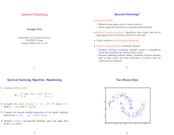
Spectral Clustering Guokun Lai 2016/10 1 / 37 Organization Graph - PowerPoint PPT Presentation
Spectral Clustering Guokun Lai 2016/10 1 / 37 Organization Graph Cut Fundamental Limitations of Spectral Clustering Ng 2002 paper (if we have time) 2 / 37 Notation We define a undirected weighted graph G ( V , E ), where V is
Spectral Clustering Guokun Lai 2016/10 1 / 37
Organization ◮ Graph Cut ◮ Fundamental Limitations of Spectral Clustering ◮ Ng 2002 paper (if we have time) 2 / 37
Notation ◮ We define a undirected weighted graph G ( V , E ), where V is the G ’s nodes set, and E is the G ’s edges set. The adjacency matrix is W ij = E ( i , j ), W ij ≥ 0. ◮ The degree Matrix D ∈ R n × n is a diagonal matrix and D i , i = � n j =1 W i , j . ◮ The Laplacian Matrix L ∈ R n × n is L = D − W . ◮ Indicator vector of a cluster: The indicator vector I c of a cluster C is , � 1 v i ∈ C I c , i = (1) 0 otherwise 3 / 37
Graph Cut The intuition of clustering is to separate points in different groups according to their similarities. If we try to separate the node set G into two disjoint sets A and B , we define � Cut ( A , B ) = w ij i ∈ A , j ∈ B If we split the node set into K disjoint set, then K � Cut ( A 1 , · · · , A k ) = Cut ( A , A ) i =1 Where A is the complement set of A . 4 / 37
Defect of Graph Cut The simplest idea to cluster the node set V is to find a partition to minimize the Graph Cut function. But usually it will lead to solutions that the subset with few nodes. 5 / 37
Normalization Cut For overcoming the defect of the Graph Cut, the Shi proposed a new cost function to regularize the size of the subset. First, we define Vol ( A ) = � i ∈ A , j ∈ V w ( i , j ), and we have Ncut ( A , B ) = cut ( A , B ) + cut ( A , B ) V ( A ) V ( B ) 6 / 37
Relation between NCut and Spectral Clustering Given a vertex subset A i ∈ V , we define the vector 1 √ f i = I A i ∗ Vol ( A i ) . Then we can write the optimization problem as, n NCut = 1 i Lf i = 1 � f T 2 Tr ( F T LF ) min 2 A i i =0 1 (2) s . t . f i = I A i ∗ � Vol ( A i ) F T DF = I 7 / 37
Optimization 1 √ Because the constraint f i = I A i ∗ Vol ( A i ) , the optimization problem is a np-hard problem. So we can relax this constraint to the R n . Then the optimization problem is, Tr ( F T LF ) min f i (3) s . t . F T DF = I Then we found the solution is the kth smallest eigenvector of D − 1 L . Based on the F , we recover the A i by the k-mean algorithm. 8 / 37
Unnormalized Laplacian Matrix Similar to the above approach, we can prove that the eigenvectors of the unnormalized Laplacian matrix is the relaxed solution for RatioCut ( A , B ) = cut ( A , B ) + cut ( A , B ) 1 √ . We can set f i = I A i ∗ | A | | B | | A i | and get the relaxed optimization problem, Tr ( F T LF ) min f i (4) s . t . F T F = I 9 / 37
Approximation The solution from the spectral method is approximately for the Normalized Cut objective function. And there is not bound for the gap between them. We can easily construct a case to make the solution to the relaxed problem very different from the origin problem. 10 / 37
Experiment Result of Shi paper 11 / 37
Organization ◮ Graph Cut ◮ Fundamental Limitations of Spectral Clustering ◮ Ng 2002 paper (if we have time) 12 / 37
Fundamental Limitations of Spectral Clustering As mentioned above, the spectral clustering approximately solve the Normalized Graph Cut objective function. But is that the Normalized Graph Cut a good criterion for the all situations? 13 / 37
Limitation of NCut The NCut function is more likely to capture the global structure. But sometimes, we may want to extract some local feature of the graph. The Graph Normalized Cut cannot separate the Gaussian distribution and the band. 14 / 37
Limitation of Spectral Clustering Next we analyze the spectral method based on the view of random walk process. We define the Markov transition matrix as M = D − 1 W , it has eigenvalue λ i and eigenvector v i . And the random walk process in the graph converges to the unique equilibrium distribution π s . Then we can found the relationship between eigenvector and the ’diffusion distance’ between points, j ( v j ( x ) − v j ( y )) 2 = || p ( z , t | x ) − p ( z , t | y ) || 2 � λ 2 t L 2 (1 /π s ) j So we see that the spectral method want to capture the major pattern of the random walk on whole graph. 15 / 37
Limitation of Spectral Clustering But this method would fail in the situation, which the scale of clusters are very different. 16 / 37
Self-Tuning Spectral Clustering One way to solve above case is that we can accelerate the random walk process in the low density area. Assume we define the distance between node is, A i , j = exp ( − d ( v i , v j ) 2 ) σ i σ j And σ i = d ( v i , v k ), where v k is the k-th nearest neighbor of v i . 17 / 37
Result of Self-Tuning Spectral Clustering 18 / 37
Failure case 19 / 37
Another solution The paper proposed a solution is that we split the graph into two subsets recursively. And stop criterion is based on the relaxation time of the graph, which is τ V = 1 / (1 − λ 2 ). ◮ Then if the size of two subsets after splitting is comparable, we expect τ V >> τ 1 + τ 2 ◮ Otherwise, we expect max ( τ 1 , τ 2 ) >> min ( τ 1 , τ 2 ). If the partition satisfy either condition, we accept separation and continue to split the subset. If not, we stop. But it didn’t address how to deal with K clustering problem. 20 / 37
Tong Zhang 2007 paper This paper gave a upper bound of expectation error in the semi-supervised learning task on graph. Because of the room of presentation, I will just introduce a interesting conclusion of this paper. 21 / 37
S-Normalized Laplacian Matrix We define the S-Normalized Laplacian Matrix as L S = S − 1 / 2 LS − 1 / 2 where S is a diagonal matrix. According to the analyze of the this paper, the best choice of S is S i , i = | C j | , where C j is the size of the cluster j . So this is an approach want to solve the different scale cluster problem cannot be dealt with by the spectral clustering. We can find this is similar to the self-tuning spectral clustering, it renormalized the adjacency matrix as ˆ W ij √ | C i | √ W ij = | C j | . 22 / 37
S-Normalized Laplacian Matrix But we don’t know | C j | , the author proposed a method to approximately computer it. We can define K − 1 = α I + L S , α ∈ R . In the ideal case, which is that we have q disjoint connected components. Then we can prove that q 1 � | C j | v j v T α → 0 , α K = j + O ( α ) i =1 where v j is the indicator vector of the cluster j . So if we have a 1 small α , we can assume K i , i ∝ | C j | . Then we can set S i , i ∝ K i , i . 23 / 37
Comparation 24 / 37
Organization ◮ Graph Cut ◮ Fundamental Limitations of Spectral Clustering ◮ Ng 2002 paper (if we have time) 25 / 37
Ng 2002 paper This paper analyzed the spectral clustering problem based on the matrix perturbation theory. It obtains a error bound of the spectral clustering algorithm with several assumptions. 26 / 37
Algorithm ◮ Define the weighted adjacency Matrix W, and construct the Laplacian Matrix L = D − 1 / 2 WD − 1 / 2 . ◮ Find x 1 , · · · , x k , the K largest eigenvectors of L, and form the matrix X = [ x 1 · · · x k ] ∈ R n ∗ k ◮ Normalized the every row of X to have unit length, j X 2 ij ) 1 / 2 Y ij = X ij / ( � ◮ Treating each row of Y as a point in R k , cluster them into k clusters via K-means. 27 / 37
Ideal Case Assume the graph G contain K clusters, and it dose not contain cross-clusters edge. In this case, the Laplacian matrix contains exactly K eigenvector with eigenvalue 1. 28 / 37
Y Matrix of Ideal Case After running the algorithm on this graph, we can get Y matrix as Where R is any rotation matrix, and each row of Y will cluster into 3 groups naturally. 29 / 37
The general case In real world data, we have cross-clusters edges. So the author analyzes the cross-clusters edges influence on the Y matrix based on the matrix perturbation theory. 30 / 37
The general case Assumption 1 There exists δ > 0 so that, for all second largest eigenvalue of each cluster, i = 1 , · · · , k , λ i 2 ≤ 1 − δ . Assumption 2 There is some fixed ǫ 1 > 0 , so that for every W 2 i 1 , i 2 ∈ 1 , · · · , k , i 1 � = i 2 , we have that � � jk d k ≤ ǫ 1 , j ∈ S i 1 k ∈ S i 2 d j ˆ ˆ where ˆ d i is the degree of i in its cluster. The intuition of this inequality is to limit the weight of cross-cluster edges, compared to weight of the intra-cluster edges. 31 / 37
The general case Assumption 3 There is some fixed ǫ 2 > 0 , so that for every j ∈ S i , we have that k �∈ Si W 2 � W 2 jk d l ) − 1 / 2 ≤ ǫ 2 ( � kl ˆ k , l ∈ S i d k ˆ ˆ d j The intuition of this inequality is also to limit the weight of cross-cluster edges, compared to weight of the intra-cluster edges. Assumption 4 There is some constant C > 0 so that for every i ≥ ( � n i i ) / ( Cn i ) . i = 1 , · · · , k , j = 1 , · · · , n i , we have ˆ k =1 ˆ d j d k The intuition of this inequality is that no points in a cluster be ”too much less” connected than other points in the same cluster. 32 / 37
The general case � k ( k − 1) ǫ + k ∗ ǫ 2 If the all of assumptions holds, set ǫ = 2 If √ σ > (2 + 2) ǫ . There exists k orthogonal vectors r 1 , · · · , r k so that k n i √ ǫ 2 1 � � || y j j − r i || 2 k ) 2 2 ≤ 4 C (4 + 2 ∗ √ n 2 ǫ ) 2 ( σ − i =1 j =1 33 / 37
Recommend
More recommend
Explore More Topics
Stay informed with curated content and fresh updates.
