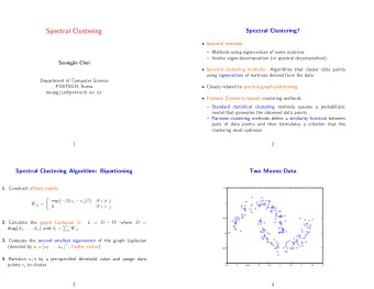
Spectral Clustering Aarti Singh Machine Learning 10-701/15-781 Nov - PowerPoint PPT Presentation

Spectral Clustering Aarti Singh Machine Learning 10-701/15-781 Nov 22, 2010 Slides Courtesy: Eric Xing, M. Hein & U.V. Luxburg 1

Data Clustering

Graph Clustering Goal: Given data points X 1 , …, X n and similarities w(X i ,X j ), partition the data into groups so that points in a group are similar and points in different groups are dissimilar. V – Vertices (Data points) Similarity Graph: G(V,E,W) E – Edge if similarity > 0 W - Edge weights (similarities) Similarity graph Partition the graph so that edges within a group have large weights and edges across groups have small weights.

Similarity graph construction Similarity Graphs: Model local neighborhood relations between data points E.g. Gaussian kernel similarity function Controls size of neighborhood W ij Data clustering

Partitioning a graph into two clusters Min-cut: Partition graph into two sets A and B such that weight of edges connecting vertices in A to vertices in B is minimum. • Easy to solve O(VE) algorithm • Not satisfactory partition – often isolates vertices

Partitioning a graph into two clusters Partition graph into two sets A and B such that weight of edges connecting vertices in A to vertices in B is minimum & size of A and B are very similar. Normalized cut: But NP-hard to solve!! Spectral clustering is a relaxation of these.

Normalized Cut and Graph Laplacian Let f = [f 1 f 2 … f n ] T with f i =

Normalized Cut and Graph Laplacian min = min where f = [f 1 f 2 … f n ] T with f i = f T D1 = 0 Relaxation: min s.t. Solution: f – second eigenvector of generalized eval problem Obtain cluster assignments by thresholding f at 0

Approximation of Normalized cut Let f be the eigenvector corresponding to the second smallest eval of the generalized eval problem. Equivalent to eigenvector corresponding to the second smallest eval of the normalized Laplacian L’ = D -1 L = I - D -1 W Recover binary partition as follows: i є A if f i ≥ 0 i є B if f i < 0 Ideal solution Relaxed solution

Example Xing et al 2001

How to partition a graph into k clusters?

Spectral Clustering Algorithm W, L’ Dimensionality Reduction n x n → n x k

Eigenvectors of Graph Laplacian • 1 st Eigenvector is the all ones vector 1 (if graph is connected) • 2 nd Eigenvector thresholded at 0 separates first two clusters from last two • k-means clustering of the 4 eigenvectors identifies all clusters

Why does it work? Data are projected into a lower-dimensional space (the spectral/eigenvector domain) where they are easily separable, say using k-means. Original data Projected data Graph has 3 connected components – first three eigenvectors are constant (all ones) on each component.

Understanding Spectral Clustering • If graph is connected, first Laplacian evec is constant (all 1s) • If graph is disconnected (k connected components), Laplacian is block diagonal and first k Laplacian evecs are: 0 0 1 L 1 … 0 0 … 0 L = 1 L 2 0 OR 0 … 1 … 0 L 3 0 0 First three eigenvectors

Understanding Spectral Clustering • Is all hope lost if clusters don’t correspond to connected components of graph? No! • If clusters are connected loosely (small off-block diagonal enteries), then 1 st Laplacian even is all 1s, but second evec gets first cut (min normalized cut) .47 .50 .50 .52 .1 .50 -.47 .50 .1 -.52 1 st evec is constant Sign of 2 nd evec since graph is connected indicates blocks

Why does it work? Block weight matrix (disconnected graph) results in block eigenvectors: Normalized to have unit norm f 2 W f 1 Slight perturbation does not change span of eigenvectors significantly: .47 .50 .50 .52 .1 .50 -.47 .50 .1 -.52 1 st evec is constant Sign of 2 nd evec since graph is connected indicates blocks

Why does it work? Can put data points into blocks using eigenvectors: f 1 .50 .47 .1 .52 .50 -.47 .50 .1 .50 -.52 f 2 f 2 W f 1 Embedding is same regardless of data ordering: f 1 .2 1 .50 .47 .2 0 1 1 -.47 .50 0 1 1 .1 .52 .50 1 .1 .1 .50 -.52 W f 1 f 2 f 2

Understanding Spectral Clustering • Is all hope lost if clusters don’t correspond to connected components of graph? No! • If clusters are connected loosely (small off-block diagonal enteries), then 1 st Laplacian even is all 1s, but second evec gets first cut (min normalized cut) • What about more than two clusters? eigenvectors f 2 , …, f k+1 are solutions of following normalized cut: Demo: http://www.ml.uni-saarland.de/GraphDemo/DemoSpectralClustering.html

k-means vs Spectral clustering Applying k-means to laplacian eigenvectors allows us to find cluster with non-convex boundaries. Both perform same Spectral clustering is superior

k-means vs Spectral clustering Applying k-means to laplacian eigenvectors allows us to find cluster with non-convex boundaries. k-means output Spectral clustering output

k-means vs Spectral clustering Applying k-means to laplacian eigenvectors allows us to find cluster with non-convex boundaries. Similarity matrix Second eigenvector of graph Laplacian

Examples Ng et al 2001

Examples (Choice of k) Ng et al 2001

Some Issues  Choice of number of clusters k Most stable clustering is usually given by the value of k that maximizes the eigengap (difference between consecutive eigenvalues)       k k k 1

Some Issues  Choice of number of clusters k  Choice of similarity choice of kernel for Gaussian kernels, choice of σ Good similarity measure Poor similarity measure

Some Issues  Choice of number of clusters k  Choice of similarity choice of kernel for Gaussian kernels, choice of σ  Choice of clustering method – k-way vs. recursive bipartite

Spectral clustering summary  Algorithms that cluster points using eigenvectors of matrices derived from the data  Useful in hard non-convex clustering problems  Obtain data representation in the low-dimensional space that can be easily clustered  Variety of methods that use eigenvectors of unnormalized or normalized Laplacian, differ in how to derive clusters from eigenvectors, k-way vs repeated 2-way  Empirically very successful