Spatial covariance-robust minimax prediction based on experimental - PowerPoint PPT Presentation
Spatial covariance-robust minimax prediction based on experimental design ideas Gunter Spoeck gunter.spoeck@uni-klu.ac.at Department of Statistics, University of Klagenfurt, Austria Overview Bayesian linear kriging. Covariance-robust minimax
Spatial covariance-robust minimax prediction based on experimental design ideas Gunter Spoeck gunter.spoeck@uni-klu.ac.at Department of Statistics, University of Klagenfurt, Austria
Overview Bayesian linear kriging. Covariance-robust minimax kriging Spatial covariance-robust minimax prediction based on experimental design ideas – p.1
Bayesian linear kriging 0.1 The model Gaussian model for the random field { Y ( x ) | x ∈ X } . Covariance function C ( x 1 , x 2 ) assumed to be known. f ( x ) T β + ǫ ( x ) Y ( x ) = f ( x ) T β E ( Y ( x ) | β ) = cov ( Y ( x 1 ) , Y ( x 2 ) | β ) = C ( x 1 , x 2 ) Prior knowledge about the trend parameter vector β : A priori distribution for β is Gaussian with E ( β ) = µ and cov ( β ) = Φ known. Spatial covariance-robust minimax prediction based on experimental design ideas – p.2
0.2 The predictor Known from Gaussian distribution theory: predictive a posteriori mean Y BK ( x 0 ) = f ( x 0 ) T ˆ ˆ 0 K − 1 ( Y dat − F ˆ β BK + c T β BK ) . The a posteriori mean of the trend parameter vector β : β BK = ( F T K − 1 F + Φ − 1 ) − 1 ˆ ( F T K − 1 Y dat + Φ − 1 µ ) Spatial covariance-robust minimax prediction based on experimental design ideas – p.3
0.3 The quality of prediction The Total Mean Squared Error of Prediction: TMSEP ( ˆ E (( Y ( x 0 ) − ˆ Y BK ( x 0 )) 2 ) = Y BK ( x 0 )) = C ( x 0 , x 0 ) + f ( x 0 ) T Φ f ( x 0 ) − k T ( K + F Φ F T ) − 1 k , where k = ( c 0 + FΦf ( x 0 )) . TMSEP ( ˆ Y BK ( x 0 )) ≤ TMSEP ( Universal Kriging ) Spatial covariance-robust minimax prediction based on experimental design ideas – p.4
0.4 Problems with kriging The covariance function cov ( Y ( x 1 ) , Y ( x 2 ) | β ) = C ( x 1 , x 2 ) is assumed to be known exactly. But generally the covariance function is just an estimate and therefore always is uncertain. Stein (1999): kriging predictor=empirical BLUP . Pilz et. al. (1997): kriging predictor=plug-in predictor. Consequence: Kriging plug-in predictor is non linear. Christensen (1991): Kriging TMSEP underestimates the true unknown TMSEP of the plug-in kriging predictor. Spatial covariance-robust minimax prediction based on experimental design ideas – p.5
0.5 Solutions Make use of the Bayesian paradigm and specify prior distributions over a space of covariance functions. How should one get prior knowledge about the covariance function? What are noninformative priors for covariance functions? Make use of the minimax principle, specify a class of plausible covariance functions and calculate a predictor in such a way that the maximum possible TMSEP becomes a minimum (Spöck, 1997, 2005). Spatial covariance-robust minimax prediction based on experimental design ideas – p.6
1 Covariance Functions The Matern class of covariance functions: 1 2 θ 2 − 1 Γ( θ 2 )( h ) θ 2 J θ 2 ( h θ,σ 2 ( h = || x 1 − x 2 || ) = σ 2 K M ) , θ 1 θ 1 where J θ 2 is the modified Bessel function of order θ 2 . θ 1 > 0 controlling the range of correlation. θ 2 > 0 a smoothness parameter (differentiability). θ,σ 2 ( h ) = σ 2 exp ( − h Exponential model ( θ 2 = 0 . 5) , K E θ 1 ) . θ,σ 2 ( h ) = σ 2 exp ( − h 2 Gaussian model ( θ 2 → ∞ ) , K G 1 ) . θ 2 Spatial covariance-robust minimax prediction based on experimental design ideas – p.7
Covariance-robust minimax kriging 2 Model f ( x ) T β + ǫ ( x ) , x ∈ X ⊂ R m Y ( x ) = f ( x ) T β E ( Y ( x ) | β, ν ) = cov ( Y ( x 1 ) , Y ( x 2 ) | β, ν ) C ν ( x 1 , x 2 ) ∈ C , ν ∈ Θ , compact = E ( β | ν ) = µ cov ( β | ν ) = Φ . Spatial covariance-robust minimax prediction based on experimental design ideas – p.8
3 Characterization of the CRMKP Restriction to linear affine predictors Y = w T Y dat + w 0 ; w ∈ R n , w 0 ∈ R} D a = { ˆ The TMSEPs for different predictors ˆ Y ∈ D a : TMSEP ( C ν ; ˆ Y ) = E β E Y 0 | β,ν (( ˆ Y − Y ( x 0 )) 2 ) = C ν ( x 0 , x 0 ) + f ( x 0 ) T Φf ( x 0 ) − 2 w T ( c 0 ,ν + FΦf ( x 0 )) = w T ( K ν + FΦF T ) w + { µ T ( f ( x 0 ) − F T w ) − w 0 } 2 . + Spatial covariance-robust minimax prediction based on experimental design ideas – p.9
In the squared marginal bias { µ T ( f ( x 0 ) − F T w ) − w 0 } 2 the covariance function does not appear. Consequence: ˆ Y M ( x 0 ) may be sought in the class of all marginally unbiased predictors Y = w T Y dat + µ T ( f ( x 0 ) − F T w ) | w ∈ R n } . D = { ˆ It is characterized by the relationship TMSEP ( C ν ; ˆ TMSEP ( C ν ; ˆ Y M ( x 0 )) = inf sup sup Y ) . ˆ C ν ∈C C ν ∈C Y ∈ D Spatial covariance-robust minimax prediction based on experimental design ideas – p.10
The definition of the minimax kriging predictor necessitates that the infima and suprema exist. We therefore suppose that the parametrization of the covariance function is continuous on the compact parameter set Θ , i.e. lim ν → ν 0 C ν ( x 1 , x 2 ) = C ν 0 ( x 1 , x 2 ) for all x 1 , x 2 ∈ X . Under this assumption TMSEP ( C ν ; ˆ Y ) , interpreted as a function of ν , is for every fixed ˆ Y ∈ D a continuous function with compact domain Θ . Lemma 6.5 of Pilz (1991) then shows that � TMSEP ( C ν ; ˆ TMSEP ( C ν ; ˆ sup Y ) = sup Y ) ξ ( dν ) , C ν ∈ C ξ ∈ Ξ Θ Spatial covariance-robust minimax prediction based on experimental design ideas – p.11
where Ξ is the set of all probability measures ξ , that are defined on the σ -algebra of the Borel sets of Θ . The equivalent new minimax problem now reads TMSEP ( C ν ; ˆ Y M ( x 0 )) = sup C ν ∈ C � TMSEP ( C ν ; ˆ inf sup Y ) ξ ( dν ) , ˆ Y ∈ D ξ ∈ Ξ Θ This minimax problem may now be solved by interchanging minimization and maximization. Spatial covariance-robust minimax prediction based on experimental design ideas – p.12
Reason: Minimax theorem of Sion (1958) The set of so-called average covariance matrices M ( ξ ) = � � � � c T c T C ξ ( x 0 , x 0 ) � C ν ( x 0 , x 0 ) 0 ,ν 0 ,ξ ξ ( dν ) = c 0 ,ν K ν c 0 ,ξ K ξ Θ is convex and compact. The convexity and compactness of this set follows from the continuity in ν of the covariance functions C ν ( x 1 , x 2 ) directly from Lemma 5.1.8 in Bandemer et al. (1978) by interpreting the average covariance matrices as information matrices from experimental design. Spatial covariance-robust minimax prediction based on experimental design ideas – p.13
The minimax theorem of Sion (1958) applies since � TMSEP ( C ν ; ˆ Y ) ξ ( dν ) = Θ C ξ ( x 0 , x 0 ) + f ( x 0 ) T Φf ( x 0 ) − 2 w T ( c 0 ,ξ + FΦf ( x 0 )) = w T ( K ξ + FΦF T ) w + is a continuous and concave function in M ( ξ ) ∈ M (Ξ) and a convex function in w ∈ R n . The average covariance matrix M ( ξ ) sought in the minimax problem and weight vector w ∈ R n are saddle points of the above integrated TMSEP . Spatial covariance-robust minimax prediction based on experimental design ideas – p.14
Interchanging supremum and infimum we see that the integrated TMSEP becomes minimal if and only if we insert for ˆ Y the Bayes kriging predictor M ( ξ ) ( x 0 ) = f ( x 0 ) T ˆ ˆ ξ ( Y dat − F ˆ 0 ,ξ K − 1 Y BK β BK M ( ξ ) + c T β BK M ( ξ ) ) M ( ξ ) = ( F T K − 1 ˆ ξ F + Φ − 1 ) − 1 ( F T K − 1 ξ Y dat + Φ − 1 µ ) . β BK Thus, the minimax predictor is characterized as that Bayesian kriging predictor ˆ Y BK M ( ξ 0 ) that maximizes M ( ξ ) ) = C ξ ( x 0 , x 0 ) + f ( x 0 ) T Φf ( x 0 ) − TMSEP ( M ( ξ ); ˆ Y BK ( c 0 ,ξ + FΦf ( x 0 )) T ( K ξ + FΦF T ) − 1 ( c 0 ,ξ + FΦf ( x 0 )) . − Spatial covariance-robust minimax prediction based on experimental design ideas – p.15
4 The Equivalence of the Minimax Problem to an Experimental Design Problem Instead of maximizing the Bayes risk in M ( ξ ) we consider here the equivalent problem of minimization of the reciprocal M ( ξ ) ) − 1 → min TMSEP ( M ( ξ ); ˆ Y BK ξ ∈ Ξ . Spatial covariance-robust minimax prediction based on experimental design ideas – p.16
If we apply the block-inversion rule to the regular, blocked matrix, in the following called average total covariance matrix, � � C ξ ( x 0 , x 0 ) + f ( x 0 ) T Φf ( x 0 ) ( c 0 ,ξ + FΦf ( x 0 )) T M b ( ξ ) = , K ξ + FΦF T c 0 ,ξ + FΦf ( x 0 ) then the first block in the inverse M b ( ξ ) − 1 is given by TMSEP ( M ( ξ ); ˆ M ( ξ ) ) − 1 , Y BK the reciprocal of the integrated Bayes kriging TMSEP . Spatial covariance-robust minimax prediction based on experimental design ideas – p.17
Multiplication of the matrix M b ( ξ ) − 1 with the unit vector c b = (1 , 0 , 0 , . . . , 0) T ∈ R n +1 in the quadratic b M b ( ξ ) − 1 c b thus results exactly in the form c T reciprokal TMSEP to be minimized. Defining M b (Ξ) = { M b ( ξ ) , ξ ∈ Ξ } , U b = c b c T b and Ψ( ξ ) = Ψ( M b ( ξ )) = tr ( U b M b ( ξ ) − 1 ) with tr ( . ) the trace operator, the minimax predictor may thus be determined by minimizing the functional Ψ( . ) in M b ( ξ ) . Ψ( M b ( ξ )) is in form equivalent to a design functional. Spatial covariance-robust minimax prediction based on experimental design ideas – p.18
Recommend
More recommend
Explore More Topics
Stay informed with curated content and fresh updates.


