sparse matrices and graphs L. Olson Department of Computer Science - PowerPoint PPT Presentation
sparse matrices and graphs L. Olson Department of Computer Science University of Illinois at Urbana-Champaign 1 objectives Convert a graph into a sparse matrix Go over a few sparse matrix storage formats Give an example of lower
sparse matrices and graphs L. Olson Department of Computer Science University of Illinois at Urbana-Champaign 1
objectives • Convert a graph into a sparse matrix • Go over a few sparse matrix storage formats • Give an example of lower memory benefits • Give an example of computational complexity benefits 2
sparse matrices • Vague definition: matrix with few nonzero entries • For all practical purposes: an m × n matrix is sparse if it has O ( min ( m , n )) nonzero entries. • This means roughly a constant number of nonzero entries per row and column 3
sparse matrices • Other definitions use a slow growth of nonzero entries with respect to n or m . • Wilkinson’s Definition: “..matrices that allow special techniques to take advantage of the large number of zero elements.” (J. Wilkinson)” • A few applications which lead to sparse matrices: Structural Engineering, Computational Fluid Dynamics, Reservoir simulation, Electrical Networks, optimization, data analysis, information retrieval (LSI), circuit simulation, device simulation, . . . 4
sparse matrices: the goal • To perform standard matrix computations economically i.e., without storing the zeros of the matrix. • For typical Finite Element /Finite difference matrices, number of nonzero elements is O ( n ) . Example To add two square dense matrices of size n requires O ( n 2 ) operations. To add two sparse matrices A and B requires O ( nnz ( A ) + nnz ( B )) where nnz ( X ) = number of nonzero elements of a matrix X . remark A − 1 is usually dense, but L and U in the LU factorization may be reasonably sparse (if a good technique is used). 5
goal • Principle goal: solve Ax = b where A ∈ R n × n , x , b ∈ R n • Assumption: A is very sparse • General approach: iteratively improve the solution • Given x 0 , ultimate “correction” is x 1 = x 0 + e 0 where e 0 = x − x 0 , thus Ae 0 = Ax − Ax 0 , • or x 1 = x 0 + A − 1 r 0 where r 0 = b − Ax 0 6
goal • Principle difficulty: how do we “approximate” A − 1 r or reformulate the iteration? • One simple idea: x 1 = x 0 + α r 0 • operation is inexpensive if r 0 is inexpensive • requires very fast sparse mat-vec (matrix-vector multiply) Ax 0 7
sparse matrices • So how do we store A ? • Fast mat-vec is certainly important; also ask • what type of access (rows, cols, diag, etc)? • dynamic allocation? • transpose needed? • inherent structure? • Unlike dense methods, not a lot of standards for iterative • dense BLAS have been long accepted • sparse BLAS still iterating • Even data structures for dense storage not as obvious • Sparse operations have low operation/memory reference ratio 8
popular storage structures DNS Dense ELL Ellpack-Itpack BND Linpack Banded DIA Diagonal COO Coordinate BSR Block Sparse Row CSR Compressed Sparse Row SSK Symmetric Skyline CSC Compressed Sparse Column BSR Nonsymmetric Skyline MSR Modified CSR JAD Jagged Diagonal LIL Linked List note: CSR = CRS, CCS = CSC, SSK = SKS in some references 9
dns 1 . 0 2 . 0 3 . 0 A = 4 . 0 5 . 0 6 . 0 7 . 0 8 . 0 9 . 0 � � AA = 3 3 1 . 0 2 . 0 3 . 0 4 . 0 5 . 0 6 . 0 7 . 0 8 . 0 9 . 0 • simple • row-wise • easy blocked formats 10
coo 1 0 0 2 0 3 4 0 5 0 A = 6 0 7 8 9 0 0 10 11 0 0 0 0 0 12 AA = [ 12 . 0 9 . 0 7 . 0 5 . 0 1 . 0 2 . 0 11 . 0 3 . 0 6 . 0 4 . 0 8 . 0 10 . 0 ] JR = [ 5 3 3 2 1 1 4 2 3 2 3 4 ] JC = [ 5 5 3 4 1 4 4 1 1 2 4 3 ] • simple, often used for entry 11
csr 1 0 0 2 0 3 4 0 5 0 A = 6 0 7 8 9 0 0 10 11 0 0 0 0 0 12 AA = [ 1 . 0 2 . 0 3 . 0 4 . 0 5 . 0 6 . 0 7 . 0 8 . 0 9 . 0 10 . 0 11 . 0 12 . 0 ] JA = [ 1 4 1 2 4 1 3 4 5 3 4 5 ] IA = [ 1 3 6 10 12 13 ] • Length of AA and JA is nnz ; length of IA is n + 1 • IA ( j ) gives the index (offset) to the beginning of row j in AA and JA (one origin due to Fortran) • no structure, fast row access, slow column access • related: CSC, MSR 12
msr 1 0 0 2 0 3 4 0 5 0 A = 6 0 7 8 9 0 0 10 11 0 0 0 0 0 12 AA = [ 1 . 0 4 . 0 7 . 0 11 . 0 12 . 0 2 . 0 3 . 0 5 . 0 6 . 0 8 . 0 9 . 0 10 . 0 ] ∗ JA = [ 7 8 10 13 14 14 4 1 4 1 4 5 3 ] • places importance on diagonal (often nonzero and accessed frequently) • first n entries are the diag • n + 1 is empty • rest of AA are the nondiagonal entries • first n + 1 entries in JA give the index (offset) of the beginning of the row (the IA of CSR is in this JA ) • rest of JA are the columns indices 13
dia 1 0 2 0 0 1 . 0 2 . 0 ∗ 3 4 0 5 0 3 . 0 4 . 0 5 . 0 � � A = 0 6 7 0 8 DIAG = 6 . 0 7 . 0 8 . 0 IOFF = − 1 0 2 0 0 9 10 0 9 . 0 10 . 0 ∗ 0 0 0 11 12 11 . 0 12 . 0 ∗ • need to know the offset structure • some entries will always be empty 14
try it... 7 0 0 0 0 0 0 1 2 0 0 0 A = 0 2 0 2 0 0 0 0 0 0 5 0 0 0 0 0 6 4 • CSR • COO 15
example i IA JA AA i IA JA AA 1 2 2 1 1 1 1 7 7 0 0 0 0 0 2 3 4 2 2 2 2 1 3 4 5 5 3 4 3 2 0 1 2 0 0 0 4 2 3 2 4 6 2 2 A = 0 2 0 2 0 0 5 5 6 4 5 7 4 2 6 1 1 7 6 9 5 5 0 0 0 0 5 0 7 5 5 6 7 - 5 6 0 0 0 0 6 4 8 3 2 2 8 - 6 4 COO CSR 16
sparse matrix-vector multiply z = Ax , A m × n , x n × 1 , z m × 1 1 input A , x 2 z = 0 3 for i = 1 to m for col = A ( i , :) 4 z ( i ) = z ( i ) + A ( i , col ) x ( col ) 5 end 6 7 end 17
sparse matrix-vector multiply z = Ax , A m × n , x n × 1 , z m × 1 1 DO I=1, m Z(I)=0 2 K1 = IA(I) 3 K2 = IA(I+1)-1 4 DO J=K1, K2 5 z(I) = z(I) + A(J)*x(JA(J)) 6 ENDDO 7 8 ENDDO • O ( nnz ) • marches down the rows • very cheap 18
sparse matrix-matrix multiply • ways to optimize (“SMPP”, Douglas, Bank) Z = AB , A m × n , B n × p , z m × p 1 for i = 1 to m for j = 1 to n 2 Z ( i , j ) = dot ( A ( i , :) , B (: , j )) 3 end 4 5 end 6 return Z • obvious problem: column selection of B is expensive for CSR • not-so-obvious problem: Z is sparse(!!), but the algorithm doesn’t account for this. 19
sparse matrix-matrix multiply Z = AB , A m × n , B n × p , z m × p 1 Z=0 2 for i = 1 to m for colA = A ( i , :) 3 for colB = A ( colA , :) 4 Z ( i , colB )+ = A ( i , colA ) · B ( colA , colB ) 5 end 6 end 7 8 end 9 return Z • only marches down rows • only computes nonzero entries in Z (aside from fortuitous subtractions) • line 5 will do and insert into Z . Two options: 1. precompute sparsity of Z in CSR 2. use LIL for Z 20
21
some python i IA JA AA 1 2 2 1 2 3 4 2 7 0 0 0 0 0 3 4 5 5 0 1 2 0 0 0 COO A = 0 2 0 2 0 0 4 2 3 2 5 5 6 4 0 0 0 0 5 0 6 1 1 7 0 0 0 0 6 4 7 5 5 6 8 3 2 2 1 from scipy import sparse 2 from numpy import array 3 IA=array([1,2,3,1,4,0,4,2]) 4 JA=array([1,3,4,2,5,0,4,1]) 5 V=array([1,2,5,2,4,7,6,2]) 6 7 A=sparse.coo_matrix((V,(IA,JA)),shape=(5,6)) 22
some python From COO to CSC: 1 from scipy import sparse 2 from numpy import array 3 import pprint 4 IA=array([1,2,3,1,4,0,4,2]) 5 JA=array([1,3,4,2,5,0,4,1]) 6 V=array([1,2,5,2,4,7,6,2]) 7 8 A=sparse.coo_matrix((V,(IA,JA)),shape=(5,6)).tocsr() Nonzeros: 1 print(A.nnz) To full and view: 1 B=A.todense() 2 pprint.pprint(B) 23
simple matrix iterations • Solve Ax = b • Assumption: A is very sparse • Let A = N + M , then Ax = b ( N + M ) x = b Nx = b − Mx • Make this into an iteration: Nx k = b − Mx k − 1 N − 1 ( b − Mx k − 1 ) x k = • Careful choice of N and M can give effective methods • More powerful iterative methods exist 24
Recommend
More recommend
Explore More Topics
Stay informed with curated content and fresh updates.
