Sparse Fuzzy Techniques There Is Room for . . . Our Idea Improve - PowerPoint PPT Presentation
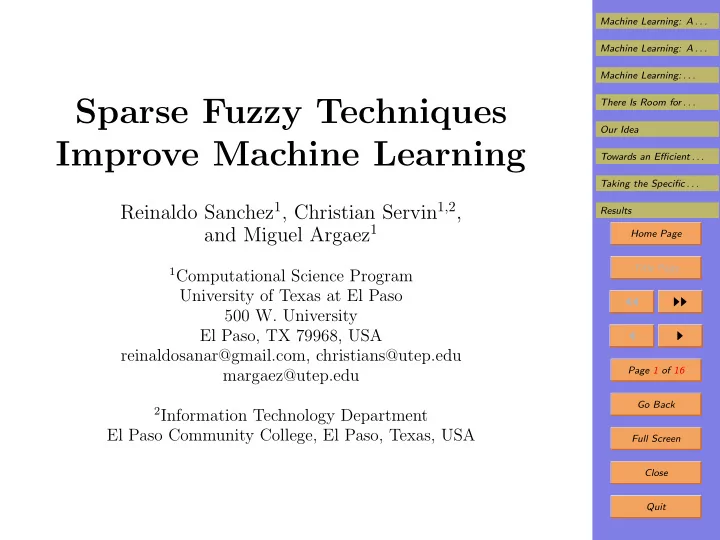
Machine Learning: A . . . Machine Learning: A . . . Machine Learning: . . . Sparse Fuzzy Techniques There Is Room for . . . Our Idea Improve Machine Learning Towards an Efficient . . . Taking the Specific . . . Reinaldo Sanchez 1 , Christian
Machine Learning: A . . . Machine Learning: A . . . Machine Learning: . . . Sparse Fuzzy Techniques There Is Room for . . . Our Idea Improve Machine Learning Towards an Efficient . . . Taking the Specific . . . Reinaldo Sanchez 1 , Christian Servin 1 , 2 , Results and Miguel Argaez 1 Home Page Title Page 1 Computational Science Program University of Texas at El Paso ◭◭ ◮◮ 500 W. University El Paso, TX 79968, USA ◭ ◮ reinaldosanar@gmail.com, christians@utep.edu Page 1 of 16 margaez@utep.edu Go Back 2 Information Technology Department El Paso Community College, El Paso, Texas, USA Full Screen Close Quit
Machine Learning: A . . . 1. Machine Learning: A Typical Problem Machine Learning: A . . . Machine Learning: . . . • In machine learning: There Is Room for . . . – we know how to classify several known objects, and Our Idea – we want to learn how to classify new objects. Towards an Efficient . . . Taking the Specific . . . • For example, in a biomedical application: Results – we have microarray data corresponding to healthy Home Page cells and Title Page – we have microarray data corresponding to different ◭◭ ◮◮ types of tumors. ◭ ◮ • Based on these samples, we would like to be able, given a microarray data, to decide Page 2 of 16 – whether we are dealing with a healthy tissue or with Go Back a tumor, and Full Screen – if it is a tumor, what type of cancer does the patient Close have. Quit
Machine Learning: A . . . 2. Machine Learning: A Formal Description Machine Learning: A . . . Machine Learning: . . . • Each object is characterized by the results x = ( x 1 , . . . , x n ) There Is Room for . . . of measuring several ( n ) different quantities. Our Idea • So, in mathematical terms, machine learning can be Towards an Efficient . . . described as a following problem: Taking the Specific . . . Results – we have K possible labels 1 , . . . , K describing dif- Home Page ferent classes; – we have several vectors x ( j ) ∈ R n , j = 1 , . . . , N ; Title Page – each vector is labeled by an integer k ( j ) ranging ◭◭ ◮◮ from 1 to K ; ◭ ◮ – vectors labeled as belonging to the k -th class will Page 3 of 16 be also denoted by x ( k, 1) , . . . , x ( k, N k ); Go Back – we want to use these vectors to assign, to each new vector x ∈ R n , a value k ∈ { 1 , . . . , K } . Full Screen Close Quit
Machine Learning: A . . . 3. Machine Learning: Original Idea Machine Learning: A . . . Machine Learning: . . . • Often, each class C k is convex : if x, x ′ ∈ C k and α ∈ There Is Room for . . . (0 , 1), then α · x + (1 − α ) · x ′ ∈ C k . Our Idea • It all C k are convex, then we can separate them by Towards an Efficient . . . using linear separators. Taking the Specific . . . Results • For example, for K = 2, there exists a linear function � n Home Page f ( x ) = c 0 + c i · x i and a threshold value y 0 such that: i =1 Title Page – for all vectors x ∈ C 1 , we have f ( x ) < y 0 , while ◭◭ ◮◮ – for all vectors x ∈ C 2 , we have f ( x ) > y 0 . ◭ ◮ • This can be used to assign a new vector x to an appro- Page 4 of 16 priate class: x → C 1 if f ( x ) < y 0 , else x → C 2 . Go Back • For K > 2, we can use linear functions separating dif- Full Screen ferent pairs of classes. Close Quit
Machine Learning: A . . . 4. Machine Learning: Current Development Machine Learning: A . . . Machine Learning: . . . • In practice, the classes C k are often not convex. There Is Room for . . . • As a result, we need nonlinear separating functions. Our Idea • The first such separating functions came from simulat- Towards an Efficient . . . ing (non-linear) biological neurons. Taking the Specific . . . Results • Even more efficient algorithms originate from the Tay- Home Page lor representation of a separating function: Title Page n n n � � � f ( x 1 , . . . , x n ) = c 0 + c i · x i + c ij · x i · x j + . . . ◭◭ ◮◮ i =1 i =1 j =1 ◭ ◮ • This expression becomes linear if we add new variables Page 5 of 16 x i · x j , etc., to the original variables x 1 , . . . , x n . Go Back • The corresponding Support Vector Machine (SVM) tech- niques are the most efficient in machine learning. Full Screen • For example, SVM is used to automatically diagnose Close cancer based on the microarray gene expression data. Quit
Machine Learning: A . . . 5. There Is Room for Improvement Machine Learning: A . . . Machine Learning: . . . • In SVM, we divide the original samples into a training There Is Room for . . . set and a training set. Our Idea • We train an SVM method on the training set. Towards an Efficient . . . Taking the Specific . . . • We test the resulting classification on a testing set. Results • Depending on the type of tumor, 90 to 100% correct Home Page classifications. Title Page • 90% is impressive, but it still means that up to 10% of ◭◭ ◮◮ all the patients are misclassified. ◭ ◮ • How can we improve this classification? Page 6 of 16 Go Back Full Screen Close Quit
Machine Learning: A . . . 6. Our Idea Machine Learning: A . . . Machine Learning: . . . • Efficient linear algorithms are based on an assumption There Is Room for . . . that all the classes C k are convex. Our Idea • In practice, the classes C k are often not convex. Towards an Efficient . . . • SVM uses (less efficient) general nonlinear techniques. Taking the Specific . . . Results • Often, while the classes C k are not exactly convex , they Home Page are somewhat convex: Title Page – for many vectors x and x ′ from each class C k and ◭◭ ◮◮ for many values α , – the convex combination α · x +(1 − α ) · x ′ still belongs ◭ ◮ to C k . Page 7 of 16 • In this talk, we use fuzzy techniques to formalize this Go Back imprecise idea of “somewhat” convexity. Full Screen • We show that the resulting machine learning algorithm Close indeed improves the efficiency. Quit
Machine Learning: A . . . 7. Need to Use Degrees Machine Learning: A . . . Machine Learning: . . . • “Somewhat” convexity means that if x, x ′ ∈ C k , then There Is Room for . . . α · x + (1 − α ) · x ′ ∈ C k with some degree of confidence. Our Idea • Let µ k ( x ) denote our degree of confidence that x ∈ C k . Towards an Efficient . . . • We arrive at the following fuzzy rule: If x, x ′ ∈ C k and Taking the Specific . . . convexity holds, then α · x + (1 − α ) · x ′ ∈ C k . Results Home Page • If we use product for “and”, we get Title Page µ k ( α · x + (1 − α ) · x ′ ) ≥ r · µ k ( x ) · µ k ( x ′ ) . ◭◭ ◮◮ • So, if x ′′ is a convex combination of two sample vectors, ◭ ◮ then µ k ( x ′′ ) ≥ r · 1 · 1 = r . Page 8 of 16 • For combination of three sample vectors, µ k ( x ′′ ) ≥ r 2 . Go Back � N k α j · x ( k, j ) , we have µ k ( y ) ≥ r � α � 0 − 1 , where • For y = Full Screen j =1 Close � α � 0 is the number of non-zero values α j . Quit
Machine Learning: A . . . 8. Using Closeness Machine Learning: A . . . Machine Learning: . . . • If y ∈ C k and x is close to y , then x ∈ C k with some There Is Room for . . . degree of confidence. Our Idea • In probability theory, Central Limit Theorem leads to Towards an Efficient . . . Gaussian degree of confidence. Taking the Specific . . . Results • We thus assume that the degree of confidence is de- � � −� x − y � 2 Home Page 2 scribed by a Gaussian expression exp . σ 2 Title Page • As a result, for every two vectors x and y , we have ◭◭ ◮◮ � � −� x − y � 2 ◭ ◮ 2 µ k ( x ) ≥ µ k ( y ) · exp . σ 2 Page 9 of 16 Go Back Full Screen Close Quit
Machine Learning: A . . . 9. Combining Both Formulas Machine Learning: A . . . Machine Learning: . . . • Resulting formula: µ k ( x ) ≥ � µ k ( x ), where: There Is Room for . . . � � 2 � � Our Idea � N k � � � x − α j · x ( k, j ) � � Towards an Efficient . . . � j =1 def · r � α � 0 − 1 . 2 µ k ( x ) � = max exp − Taking the Specific . . . σ 2 α Results Home Page Title Page • To classify a vector x , we: ◭◭ ◮◮ – compute � µ k ( x ) for different classes k , and ◭ ◮ – select the class k for which � µ k ( x ) is the largest. Page 10 of 16 • This is equivalent to minimizing L k ( x ) = − ln( � µ k ( x )): Go Back � � 2 � � N k � � � Full Screen L k ( x ) = C · � x − α j · x ( k, j ) + � α � 0 . � � � j =1 Close 2 Quit
Recommend
More recommend
Explore More Topics
Stay informed with curated content and fresh updates.


