Space-efficient quantum Space-efficient quantum automata automata - PowerPoint PPT Presentation
Space-efficient quantum Space-efficient quantum automata automata Andris Ambainis Nikolay Nahimov Department of Computer Science University of Latvia TQC 2008 Quantum Finite Automata Mathematical model for quantum computers with
Space-efficient quantum Space-efficient quantum automata automata Andris Ambainis Nikolay Nahimov Department of Computer Science University of Latvia TQC 2008
Quantum Finite Automata � Mathematical model for quantum computers with limited memory � Recognize the same set of languages as DFA (deterministic finite automata) � Can be exponentially more space-efficient TQC 2008 2
Computational problem = ≡ ∈ j L { a | j 0 (mod p ) , p P } p � DFA requires O(p) states ... p states � QFA requires O(log(p)) states TQC 2008 3
Known results � A. Ambainis, R. Freivalds “1-way quantum finite automata: strengths, weaknesses and generalizations” � A. Ambainis, N. Nahimovs “Improved constructions of quantum automata” TQC 2008 4
Improvements � Simpler construction with better constant in front of log (p) and with a much simpler analysis. � A simple rule for derandomization of automata construction. TQC 2008 5
Construction steps � Define simple 2-state QFA U k depending on single parameter k � Take c·log (p) automata U k with different k TQC 2008 6
Construction: building blocks � Q = {q 0 , q 1 }, Q acc = {q 0 }, Q rej = {q 1 } � Starting state q 0 � Left and right endmarker leaves state unchanged q 0 q 1 TQC 2008 7
Construction: building blocks � Reading 'a' performs U k state “rotation” → φ + φ q cos q sin q 0 k 0 k 1 → − φ + φ q sin q cos q 1 k 0 k 1 π 2 k φ = where k p � Parameter k represents a rotation frequency TQC 2008 8
Construction: building blocks � After reading a j the state of U k is π π 2 k j 2 k j + cos q sin q 0 1 p p ⎛ ⎞ π 2 k j � Accepts a j with probability ⎜ ⎟ cos 2 ⎜ ⎟ p ⎝ ⎠ TQC 2008 9
Construction: building blocks � After reading a j the state of U k is π π 2 k j 2 k j + cos q sin q 0 1 p p ⎛ ⎞ π 2 k j � Accepts a j with probability ⎜ ⎟ cos 2 ⎜ ⎟ p ⎝ ⎠ � If accepts a j with probability 1 a ∈ j L p TQC 2008 10
Construction � Take d = c·log(p) automata U k with different k U k1 q 1,0 q 1,1 U k2 q 2,0 q 2,1 d=c·log (p) ... U kd q d,0 q d,1 TQC 2008 11
Construction q � Start at equal state superposition i , 0 ( ) 1 ϕ = + + + q q ... q start 1 , 0 2 , 0 d , 0 d U q 1,0 q 1,1 q 2,0 q 2,1 … q d,0 q d,1 TQC 2008 12
Construction q � Start at equal state superposition i , 0 ( ) 1 ϕ = + + + q q ... q start 1 , 0 2 , 0 d , 0 d q � Alternative view: start at and on the left 1 , 0 endmarker perform a transformation ( ) 1 → + + + q q q ... q 1 , 0 1 , 0 2 , 0 d , 0 d TQC 2008 13
Construction � Transformation for 'a' is as before → φ + φ q cos q sin q i , 0 k i , 0 k i , 1 i i π 2 k i φ = → − φ + φ where q sin q cos q k i i , 1 k i , 0 k i , 1 p i i U q 1,0 q 1,1 q 2,0 q 2,1 … q d,0 q d,1 TQC 2008 14
Construction � Transformation for 'a' is as before → φ + φ q cos q sin q i , 0 k i , 0 k i , 1 i i π 2 k i φ = → − φ + φ where q sin q cos q k i i , 1 k i , 0 k i , 1 p i i � After reading a j the state of U is ⎛ π π ⎞ 1 2 k j 2 k j ∑ ⎜ ⎟ + cos i q sin i q ⎜ ⎟ i , 0 i , 1 p p d ⎝ ⎠ i TQC 2008 15
Construction � Measure difference from initial state ( ) 1 ϕ = + + + q q ... q start 1 , 0 2 , 0 d , 0 d U q 1,0 q 1,1 q 2,0 q 2,1 … q d,0 q d,1 TQC 2008 16
Construction � Measure difference from initial state ( ) 1 ϕ = + + + q q ... q start 1 , 0 2 , 0 d , 0 d � Alternative view: on the right endmarker perform transformation 1 ∑ → + α q q q i , 0 1 , 0 j j , 0 d j and measure if state is q 1 , 0 TQC 2008 17
Construction � Accepts a j with probability 2 ⎞ ⎛ π π π 1 2 k j 2 k j 2 k j ⎜ ⎟ + + + cos 1 cos 2 ... cos d ⎟ ⎜ 2 d p p p ⎝ ⎠ a ∈ j j L a � If accepts with probability 1 p a ∉ j L � If we want probability to be small p TQC 2008 18
Theorem For any ε > 0 and p ∈ P, there exist k 1 ,k 2 ,...,k d ⎡ ⋅ ⎤ 2 log ( 2 p ) = , that for all j ∈ {1, ..., p-1} d ⎢ ⎥ ε ⎢ ⎥ 2 ⎞ ⎛ π π π 1 2 k j 2 k j 2 k j ⎜ ⎟ + + + < ε cos 1 cos 2 ... cos d ⎟ ⎜ 2 d p p p ⎝ ⎠ TQC 2008 19
Notes on the theorem proof � Proof is by a probabilistic argument. It applies sequence of parameters k 1 ,k 2 ,...,k d that are chosen at random. � Proof does not give an explicit parameter sequence. � A deterministic sequence construction rule is required. TQC 2008 20
Derandomization hypothesis If g is a primitive root modulo p ∈ P * , then = ≡ i d S { k g mod p } sequence for all d = g i i 1 and all j ∈ {1, ..., p-1} satisfies 2 ⎞ ⎛ π π π 1 2 k j 2 k j 2 k j ⎜ ⎟ + + + < ε cos 1 cos 2 ... cos d ⎟ ⎜ 2 d p p p ⎝ ⎠ * All g i (mod p), i ∈ {0, ..., p-1}, are different TQC 2008 21
Notation � We will refer S g = {g i (mod p)} as cyclic sequence and g as the sequence generator. � We will also use S rand to denote a random sequence. TQC 2008 22
Hypothesis check � We have checked all p ∈ {2, …, 9973} � For each p all generators g � For each p and g all sequence lengths d < p choosing a corresponding ε value � We haven't found any counterexample. TQC 2008 23
Random vs. cyclic sequences � In 99.98% - 99.99% of our experiments, random sequences achieved the bound of theorem. � For randomly selected p ∈ P, ε > 0 and generator g, a cyclic sequence S g gives a better result than a random sequence S rand in 98.29% of cases. TQC 2008 24
Random vs. cyclic sequences � Probability of error for different p, ε and g p e g e_rand e_g 1523 0.1 948 0.03635 0.01517 2689 0.1 656 0.03767 0.0195 3671 0.1 2134 0.03803 0.02122 4093 0.1 772 0.03822 0.01803 5861 0.1 2190 0.03898 0.01825 6247 0.1 406 0.03922 0.02006 7481 0.1 6978 0.03932 0.01691 8581 0.1 5567 0.03942 0.02057 9883 0.1 1260 0.04011 0.01905 TQC 2008 25
Different generators � Every p ∈ P might have multiple generators. � Different generators give QFA with different probabilities of error. One with a minimal error will be referred as a minimal generator. � Typically, the minimal generator give a QFA with a substantially smaller probability of error. TQC 2008 26
Different generators � Minimal generators for different p p e g e_g g_min e_g_min 1523 0.1 948 0.01517 624 0.00919 2689 0.1 656 0.0195 1088 0.0106 3671 0.1 2134 0.02122 1243 0.01121 4093 0.1 772 0.01803 1063 0.01154 5861 0.1 2190 0.01825 5732 0.01133 6247 0.1 406 0.02006 97 0.01182 7481 0.1 6978 0.01691 2865 0.01205 8581 0.1 5567 0.02057 4362 0.01335 9883 0.1 1260 0.01905 5675 0.01319 TQC 2008 27
Open questions � Strict mathematical proof of derandomization hypothesis. � Is it possible to find a minimal generator without an exhaustive search of all generators ? � Can other functions be represented in a similar way ? TQC 2008 28
Thank you! Thank you!
Recommend
More recommend
Explore More Topics
Stay informed with curated content and fresh updates.
