Sorting methods Classification of sorting algorithms internal vs - PowerPoint PPT Presentation

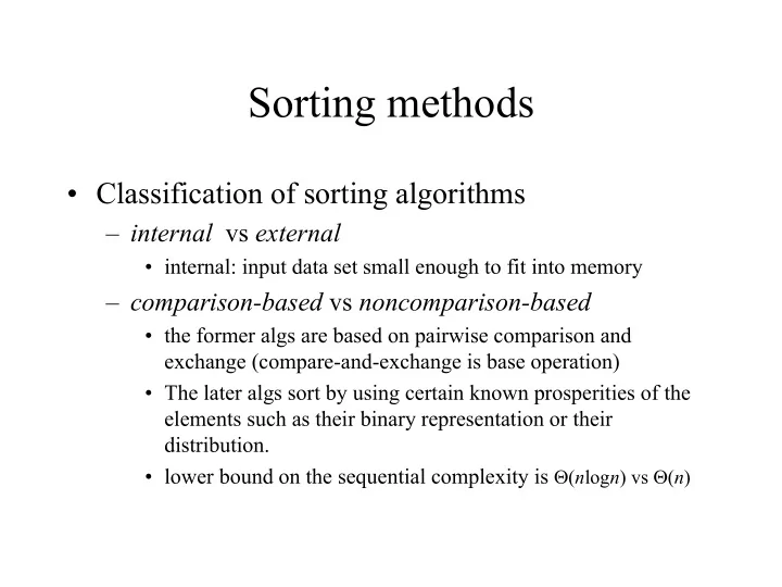
Sorting methods • Classification of sorting algorithms – internal vs external • internal: input data set small enough to fit into memory – comparison-based vs noncomparison-based • the former algs are based on pairwise comparison and exchange (compare-and-exchange is base operation) • The later algs sort by using certain known prosperities of the elements such as their binary representation or their distribution. • lower bound on the sequential complexity is Θ ( n log n ) vs Θ ( n )

Basic sorting operations: compare-exchange • Problem: how to perform compare-exchange on a parallel system with one element per processor • Solution: send element to other node, then perform comparison • Running time: – T tot = t comp + t comm – t comm = t s + t w ≈ t s (assuming neighboring nodes)

Basic sorting operations: compare-split • Problem: how to perform compare-exchange on a parallel system with n/p elements per processor • Solution: send elements to other node, then merge and retain only half of the elements • Running time: – T tot = t comp + t comm – t comm = t s + n/p t w ≈ n/p t w (neighboring nodes, n>>p )

Bubble sort • The serial version compares all adjacent Procedure BUBBLE_SORT(n) pairs in order: begin for i := 1 to n-1 do – (a 1 , a 2 ), (a 2 , a 3 ), …, (a n-1 , a n ) for j := 0 to n-i-1 do – iterate n times compare-exchange ( a j , a j+1 ) – complexity: Θ ( n 2 ) end • Some modification to base algorithm needed for parallelization Procedure ODD_EVEN(n) begin • Odd-Even Transposition: perform for i := 1 to n do compare-exchange on odd elements, then begin on even elements if i is odd then – (a 1 , a 2 ), (a 3 , a 4 ), …, (a n-1 , a n ) for j := 1 to n/2 - 1 do – (a 2 , a 3 ), (a 4 , a 5 ), …, (a n-2 , a n-1 ) compare-exchange ( a 2j+1 , a 2j+2 ) if i is even then – iterate n times for j := 1 to n/2 - 1 do – complexity: Θ ( n 2 ) compare-exchange ( a 2j , a 2j+1 ) endfor end

Odd-Even transposition example

Parallel bubble sort • Assume ring interconnect Procedure ODD_EVEN_PAR(n) • Simple case: p = n begin – Running time: Θ ( n ) id : = processor’s label • n iterations, one compare-exchange per for i := 1 to n do iteration (complexity: Θ (1)) begin – Cost: Θ ( n 2 ) if i is odd then if id is odd then • not cost optimal - compare to Θ ( n log n ) compare-exchange_min ( id + 1) • General case: p < n else – Running time: Θ ( n/p log n/p ) + Θ ( n ) compare-exchange_max(id - 1 ) • each processor sorts internally its block of if i is even then n/p element (for example using quicksort- if id is even then complexity: Θ ( n/p log n/p )) compare-exchange_min ( id + 1) • p phases each with else – Θ ( n/p ) comparisons (to merge blocks) compare-exchange_max(id - 1 ) – Θ ( n/p ) communication time endfor E = 1/(1 - Θ ((log p )/(log n )) + Θ (( p )/(log n )) ) – end i.e. cost-optimal when p = O (log n)

Quicksort Procedure QUICKSORT( A, q, r ) • The recursive algorithm consists of four steps (which closely resemble the merge sort): begin if q<r then – If there are one or less elements in the array to be sorted, return immediately. begin – Pick an element in the array to serve as a x := A [ q ] "pivot" point. (Usually the left-most element in s := q the array is used.) for i := q + 1 to r do – Split the array into two parts - one with if A [ i ] ≤ x then elements larger than the pivot and the other begin with elements smaller than the pivot. s := s + 1 – Recursively repeat the algorithm for both halves of the original array. swap ( A [ s ], A [ i ]) • Performance is affected by the way the end algorithm splits the sequence swap ( A [ q ], A [ s ]) – worst case (1 and k -1 splitting): recurrent QUICKSORT ( A, q, s ) relations QUICKSORT ( A, s + 1 , r ) • T(n) = T(n-1)+ Θ ( n ) => T(n) = Θ ( n 2 ) endif – best case ( k /2 and k /2 splitting): end • T(n) = 2T(n/2)+ Θ ( n ) => T(n) = Θ ( n log n )

Quicksort example Example

Quicksort efficient parallelization • Drawback of naïve approach: the initial partitioning of A[ q … r ] is done by a single processor – run time is bounded below by O( n ) – cost is O( n 2 ) therefore not cost-optimal • Complexity of quicksort algorithm: – T(n) = 2T(n/2)+ Θ ( n ) => Θ ( n log n ) (for optimal pivot selection) • the term Θ ( n ) is due to the partitioning – the same term could become Θ (1) if we find a way of parallelizing the partitioning using n processors • will see solutions for PRAM and hypercube

Shared memory machine: PRAM model • Parallel Random Access Machine (PRAM) is a popular model used in the design of parallel algorithms – It assumes a number of processors with a single shared memory – Variants based on concurrency of accesses: • EREW: Exclusive Read, Exclusive Write • CREW: Concurrent Read, Exclusive Write • CRCW: Concurrent Read, Concurrent Write

Parallel version on a PRAM (1) • The execution of the algorithm can be represented with a tree – the root is the initial pivot – each level represents a different iteration • If pivot selection is optimal, the height of the tree is Θ (log n ) • The parallel algorithm proceeds by selecting an initial pivot, then partitioning the array in two parts in parallel

Parallel version on a PRAM (2) • We will consider a CRCW PRAM – concurrent read, concurrent write parallel random access machine – when two or more processors write to a common location only one arbitrarily chosen is successful • The algorithm is based on two shared arrays, leftchild and rightchild , where all processors write at each iteration – the CRCW arbitration mechanism is used to pick the next pivot – average depth of the tree is Θ (log n ), each step takes Θ (1), thus – average complexity is Θ (log n ) – average cost is Θ ( n log n ) => cost optimal

1 2 3 4 5 6 7 8 1 2 3 4 5 6 7 8 33 21 13 54 82 33 40 72 (a) leftchild 1 rightchild 5 (c) root = 4 (b) 1 2 3 4 5 6 7 8 1 2 3 4 5 6 7 8 leftchild 2 1 8 leftchild 2 3 1 8 (d) (e) rightchild 6 5 rightchild 6 5 7 [4] {54} 1 2 5 8 3 6 7 (f) [1] {33} [5] {82} 2 3 6 7 8 [2] {21} [8] {72} [6] {33} 3 7 [3] {13} [7] {40} Figure 9.17 The execution of the PRAM algorithm on the array shown in (a). The arrays leftchild and rightchild are shown in (c), (d), and (e) as the algorithm progresses. Figure (f) shows the binary tree constructed by the algorithm. Each node is labeled by the process (in square brackets), and the element is stored at that process (in curly brackets). The element is the pivot. In each node, processes with smaller elements than the pivot are grouped on the left side of the node, and those with larger elements are grouped on the right side. These two groups form the two partitions of the original array. For each partition, a pivot element is selected at random from the two groups that form the children of the node.

Hypercube Sequence of Elements 100 110 (a) Split along the third 000 010 dimension. Partitions the sequence into two 0** 1** 101 111 big blocks−one smaller and one larger than the 011 001 pivot. 110 100 (b) Split along the second 000 010 01* 11* dimension. Partitions each subblock into two smaller 101 111 subblocks. 00* 10* 011 001 100 110 (c) Split along the first 000 010 010 111 dimension. The elements 011 110 are sorted according to 111 101 the global ordering imposed by the processors’ labels 000 001 100 101 011 001 onto the hypercube. Figure 9.21 The execution of the hypercube formulation of quicksort for d = 3 . The three splits – one along each communication link – are shown in (a), (b), and (c). The second column represents the partitioning of the n -element sequence into subcubes. The arrows between subcubes indicate the movement of larger elements. Each box is marked by the binary representation of the process labels in that subcube. A ∗ denotes that all the binary combinations are included.

Parallel version on hypercube • This algorithm exploits one property of hypercubes: – a d -dimensional hypercube can be split in two ( d -1)-dimensional hypercubes with the corresponding nodes directly connected – n elements are distributed on p = 2 d processors ( n/p elements per processor) • At each iteration, pivot is chosen and broadcast to all processors in same hypercube – then smaller-than-pivot elements are sent to half hypercube, the larger ones to the other half • Selection of good pivot is crucial to maintain good load balance – a good criterion is to choose the median element of an arbitrarily selected processor in the hypercube (works well with uniform distribution)

Hypercube algorithm

Hypercube algorithm complexity • The algorithms performs d iterations, each has three steps – pivot selection => Θ (1) if p/n elements are presorted – broadcast of pivot => Θ (log n ) – Tp = Θ ( n/p log n/p ) sort + Θ ( n/p log p ) comm + Θ (log 2 p ) pivot broadcasting local • Efficiency and cost-optimality analysis – E = 1/(1 - Θ ((log p )/(log n )) + Θ (( p log 2 p )/( n log n ))) – cost-optimal if Θ (( p log 2 p )/( n log n )) = O (1), i.e. can use up to p = Θ (n/ log n ) processors efficiently