SOME STATISTICAL TESTS Overview Theory of statistical tests Test - PowerPoint PPT Presentation
R course Tuesday, March 12 2013 SOME STATISTICAL TESTS Overview Theory of statistical tests Test for a difference in mean Test for dependence Nominal variables Continuous variables Ordinal variables Power of a test
R course Tuesday, March 12 2013 SOME STATISTICAL TESTS
Overview ● Theory of statistical tests ● Test for a difference in mean ● Test for dependence – Nominal variables – Continuous variables – Ordinal variables ● Power of a test ● Degrees of freedom
Overview ● Theory of statistical tests ● Test for a difference in mean ● Test for dependence – Nominal variables – Continuous variables – Ordinal variables ● Power of a test ● Degrees of freedom
Theory of statistical tests ● Read the § from the lecture notes
Overview ● Theory of statistical tests ● Test for a difference in mean ● Test for dependence – Nominal variables – Continuous variables – Ordinal variables ● Power of a test ● Degrees of freedom
Test for a difference in mean : T test ● Underline of the test – What is given? Independent observations ( x1 , . . . , xn ) and ( y1 , . . . , ym ). – Null hypothesis: x and y are samples from distributions having the same mean. – Test: t-test – R command: t.test( x, y ) – Idea of the test: If the sample means are too far apart, then reject the null hypothesis. – Approximative test but rather robust
Test for a difference in mean : T test > mars <- read.table("mars.txt",header=TRUE) ● Ex 1: marsians > head(mars) size color 1 65.67974 red – Dataset containing 2 65.90436 red 3 67.34730 red height for marsians of 4 60.42924 red 5 55.34526 red different colors 6 62.85024 red > attach(mars) – Reject the null hypo > t.test(size[color=="green"],size[color=="blue"]) – It was an unpaired t Two Sample t-test data: size[color == "green"] and size[color == "blue"] test (no dependence t = -3.4244, df = 19.419, p-value = 0.002775 alternative hypothesis: true difference in means is not between the 2 equal to 0 95 percent confidence interval: samples) -16.875514 -4.083647 sample estimates: mean of x mean of y 60.86840 71.34798
Test for a difference in mean : T test > mars <- read.table("mars.txt",header=TRUE) ● Ex 1: marsians > head(mars) size color 1 65.67974 red – Dataset containing 2 65.90436 red 3 67.34730 red height for marsians of 4 60.42924 red 5 55.34526 red different colors 6 62.85024 red > attach(mars) – Reject the null hypo > t.test(size[color=="green"],size[color=="blue"]) – It was an unpaired t Two Sample t-test data: size[color == "green"] and size[color == "blue"] test (no dependence t = -3.4244, df = 19.419, p-value = 0.002775 alternative hypothesis: true difference in means is not between the 2 equal to 0 95 percent confidence interval: samples) -16.875514 -4.083647 sample estimates: mean of x mean of y 60.86840 71.34798
Test for a difference in mean : T test ● Ex 2: shoe wear > data(shoes,package=’MASS’) > attach(shoes) > head(shoes) – Dataset containing $A [1] 13.2 8.2 10.9 14.3 10.7 6.6 9.5 10.8 8.8 wear of shoes of 2 13.3 materials A and B $B [1] 14.0 8.8 11.2 14.2 11.8 6.4 9.8 11.3 9.3 – Paired test because 13.6 > t.test(A,B,paired=TRUE) some boys will cause more damage to the Paired t-test data: A and B shoe than others t = -3.3489, df = 9, p-value = 0.008539 alternative hypothesis: true difference in – Reject the null hypo means is not equal to 0 95 percent confidence interval: -0.6869539 -0.1330461 sample estimates: mean of the differences -0.41
Test for a difference in mean : T test ● Ex 2: shoe wear > data(shoes,package=’MASS’) > attach(shoes) > head(shoes) – Dataset containing $A [1] 13.2 8.2 10.9 14.3 10.7 6.6 9.5 10.8 8.8 wear of shoes of 2 13.3 materials A and B $B [1] 14.0 8.8 11.2 14.2 11.8 6.4 9.8 11.3 9.3 – Paired test because 13.6 > t.test(A,B,paired=TRUE) some boys will cause more damage to the Paired t-test data: A and B shoe than others t = -3.3489, df = 9, p-value = 0.008539 alternative hypothesis: true difference in – Reject the null hypo means is not equal to 0 95 percent confidence interval: -0.6869539 -0.1330461 sample estimates: mean of the differences -0.41
Test for a difference in mean : T test ● Linked tests that might be of interest – var.test() to test for equality in variance → this way you can change the option var.equal in t.test() – shapiro.test() to test for normality for example before doing a Pearson correlation The null hypothesis of the shapiro test is normal distribution
Overview ● Theory of statistical tests ● Test for a difference in mean ● Test for dependence – Nominal variables – Continuous variables – Ordinal variables ● Power of a test ● Degrees of freedom
Test for dependence ● The test depends from the data type – Nominal variables (not ordered like eye color or gender) – Ordinal variables (ordered but not continuous like result of a dice) – Continuous variables (like body height)
Overview ● Theory of statistical tests ● Test for a difference in mean ● Test for dependence – Nominal variables – Continuous variables – Ordinal variables ● Power of a test ● Degrees of freedom
Test for dependence Nominal (count) variables ● Underline of the test – What is given? Pairwise observations (x1 , y1 ), ( x2 , y2 ), . . . , ( xn , yn ) – Null hypothesis: x and y are independent – Test: χ 2 -test for independence – R command: chisq.test( x, y ) or chisq.test( contingency.table ) – Idea of the test: Calculate the expected abundancies under the assumption of independence. If the observed abundancies deviate too much from the expected abundancies, then reject the null hypothesis. – Approximate test, see the conditions on the lecture notes
Test for dependence Nominal (count) variables ● Ex 1: χ 2 -test > contingency <- matrix( c(47,3,8,42,60,15,8,33,3), nrow=3 ) > chisq.test(contingency)$expected [,1] [,2] [,3] [1,] 25.689498 51.82192 19.488584 [2,] 25.424658 51.28767 19.287671 [3,] 6.885845 13.89041 5.223744 # expected abundancies are all above 5, so we may apply the test > chisq.test(contingency) Pearson’s Chi-squared test data: contingency X-squared = 58.5349, df = 4, p-value = 5.892e-12 ● Reject the null hypo that the two variables are independent
Test for dependence Nominal (count) variables ● Fisher´s exact test – 2*2 contingency tables – Example: > table <- matrix( c(14,10,21,3), nrow=2 ) > fisher.test(table) Fisher’s Exact Test for Count Data data: table p-value = 0.04899 alternative hypothesis: true odds ratio is not equal to 1 95 percent confidence interval: 0.03105031 0.99446037 sample estimates: odds ratio 0.2069884 ● We reject the null hypo
Overview ● Theory of statistical tests ● Test for a difference in mean ● Test for dependence – Nominal variables – Continuous variables – Ordinal variables ● Power of a test ● Degrees of freedom
Test for dependence Continuous variables ● Underline of the test – What is given? Pairwise observations ( x1 , y1 ), ( x2 , y2 ), . . . , ( xn , yn ); all values in some interval are possible – Null hypothesis: x and y are independent – Test: Pearson’s correlation test for independence – Assumption: x and y are samples from a normal distribution – R command: cor.test( x, y )
Test for dependence Continuous variables ● Ex: > data(cars) > attach(cars) – Distance needed to > str(cars) > ?cars stop from a certain > plot(speed,dist) speed for cars > cor.test(speed, dist) Pearson’s product-moment correlation – Reject the null hypo data: speed and dist t = 9.464, df = 48, p-value = 1.49e-12 alternative hypothesis: true correlation is not equal to 0 95 percent confidence interval: 0.6816422 0.8862036 sample estimates: cor 0.8068949
Test for dependence Continuous variables ● Ex: > data(cars) > attach(cars) – Distance needed to > str(cars) > ?cars stop from a certain > plot(speed,dist) speed for cars > cor.test(speed, dist) Pearson’s product-moment correlation – Reject the null hypo data: speed and dist t = 9.464, df = 48, p-value = 1.49e-12 alternative hypothesis: true correlation is not equal to 0 95 percent confidence interval: 0.6816422 0.8862036 sample estimates: cor 0.8068949
Overview ● Theory of statistical tests ● Test for a difference in mean ● Test for dependence – Nominal variables – Continuous variables – Ordinal variables ● Power of a test ● Degrees of freedom
Test for dependence Ordinal variables ● Underline of the test > data(cars) > attach(cars) – What is given? Pairwise > cor.test(speed, dist, method=”spearman”) observations ( x1 , y1 ), Spearman's rank correlation rho ( x2 , y2 ), . . . , ( xn , yn ); values can be ordered data: speed and dist S = 3532.819, p-value = 8.825e-14 – Null hypothesis: x and y alternative hypothesis: true rho is not equal to 0 are uncorrelated sample estimates: – Test: Spearman’s rank rho 0.8303568 correlation rho – R command: cor.test( x, Warning message: In cor.test.default(speed, dist, method = y, method="spearman") "spearman") : Cannot compute exact p-values with ties
Recommend
More recommend
Explore More Topics
Stay informed with curated content and fresh updates.
