Some Node Degree Properties of Series-Parallel Graphs Evolving Under - PowerPoint PPT Presentation

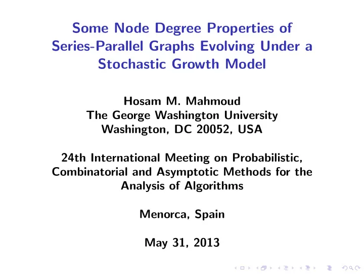
Some Node Degree Properties of Series-Parallel Graphs Evolving Under a Stochastic Growth Model Hosam M. Mahmoud The George Washington University Washington, DC 20052, USA 24th International Meeting on Probabilistic, Combinatorial and Asymptotic Methods for the Analysis of Algorithms Menorca, Spain May 31, 2013

Series-parallel (SP) graphs Series-parallel (SP) graphs are network models that can represent the flow of, for example, commercial goods from a source to a market. Consider them directed and the smallest is K 2 . N • ❄ • S

N • ❄ • N ✁ ❆ • ❍❍ ☛ ✁ ❯ ❆ ❥ • • • ❄ ✟ ✟ ✙ ❆ ✁ • ❆ ❯ ☛ ✁ • S N • S ❍❍ ❍ ❥ • ❄ ✟ N ✟ ✙ PPPPPP • • • ❆ ❄ ❆ P q • ❯ ❆ • ✑ ✁ ❆ • ✁ ✑ ✁ ☛ ✁ ❯ ❆ ✑ ✁ ✑ ✰ ☛ ✁ ✏ • • • ✭ ✁ ✭ ✏ • ✭ ❄ ✁ ☛ ✭ ❆ ✁ ✏ ✮ ✏ ✭ ✭ • ❯ ❆ ☛ ✁ • S S Figure: Two directed series-parallel graphs on top, and a graph obtained by a series composition (bottom left), and another graph obtained by their parallel composition (bottom right).

Models of randomness To the best of our knowledge, these networks have been studied under two models of randomness: ◮ the uniform model, where all SP networks of a certain size are equally likely Bernasconi, N., Panagiotou, K. and Steger, A. (2008). Drmota, M., Gim´ enez, O. and Noy, M. (2010).

Models of randomness To the best of our knowledge, these networks have been studied under two models of randomness: ◮ the uniform model, where all SP networks of a certain size are equally likely Bernasconi, N., Panagiotou, K. and Steger, A. (2008). Drmota, M., Gim´ enez, O. and Noy, M. (2010). ◮ The hierarchical lattice model Hambly, B. and Jordan, J. (2004).

Hierarchical lattice model • • �� �� p • • = ⇒ �� �� • • • • • • 1 − p • = ⇒ • • • • Figure: Hierarchical lattice model, growing too quickly.

An incremental model of randomness Starting with a directed K 2 (with its sole edge directed from the North to the South Pole), we grow an SP graph in steps. At each step, we choose an edge from the existing graph at random (all edges being equally likely). We subject that edge to either a series extension with probability p , or a parallel doubling with probability q := 1 − p .

Edge extension and doubling ◮ series extension: u • u • ❄ p • x = ⇒ ❄ • ❄ ❄ v • v ◮ Parallel doubling: u u • • �� 1 − p ❄ = ⇒ ◆ ✌ • • v v Henceforth “random” will always mean this model.

Degrees of certain nodes We look at certain node degrees in a random SP graph: ◮ The degree of a pole. We find its exact distribution, given by a probability formula with alternating signs. ◮ For a fixed number s , we study the numbers of nodes of outdegree 1 , . . . , s : asymptotically have a joint multivariate normal distribution. P´ olya urns will systematically provide a working tool.

The degree of a pole The number of edges coming out of the North Pole is a measure of the volume of trading and and the amount of goods that can be shipped out of the source. This number is the North Pole’s outdegree (it is also its degree). Polya urn Suppose we colored the edges coming out of the North Pole with white (W), and all the other edges with blue (B). We think of the edges as balls in a P´ olya urn. Let W n be the number of white balls in the urn after n edge additions to K 2 . As we start from a directed K 2 , we have W 0 = 1, and B 0 = 0.

Picking White N N • • ✟ ❍❍ ❍❍ ✟ ❍❍ ❍❍ p ✟ ✙ � ❅ ❥ ❥ ✟ ✙ � ❅ ❥ ❥ = ⇒ � ✠ ❘ ❅ � ✠ ❘ ❅ ❄ ❄ • ⋆ ❄ N N • • ✟ ❍❍ ❍❍ ✟ ❍❍ ❍❍ 1 − p ✟ ✙ � ❅ ❥ ❥ ✙ ✟ � ❅ ❏ ❥ ❥ ⇒ = ❏❍ � ✠ ❅ ❘ � ✠ ❅ ❘ ❄ ❄ ❥ ❍ • ⋆ Figure: Picking a white edge (ball).

Picking Blue • • ✟ ❍❍ ❍❍ ✟ ❍❍ ❍❍ p ✟ ✙ � ❅ ❥ ❥ ✟ ✙ � ❅ ❥ ❥ = ⇒ ✠ � ❘ ❅ � ✠ ❘ ❅ ❄ ❄ • ⋆ ❄ • • ✟ ❍❍ ❍❍ ✟ ❍❍ 1 − p ✟ ✙ � ❅ ❥ ❥ ✟ ✙ � ❅ ❏ ❥ ⇒ = ❏❍ ✠ � ❘ ❅ ✠ � ❘ ❅ ❄ ❄ ❥ ❍ • ⋆ Figure: Picking a blue edge (ball).

Dynamics of the P´ olya urn The dynamics of a two-color P´ olya urn scheme are often represented with a replacement matrix, the rows and columns of which are indexed with the two colors, and the entries are the number of balls added. The replacement matrix associated with our urn is � 1 − Ber ( p ) Ber ( p ) � 0 1 C´ ecile Mailler told us yesterday that triangular arrays have a special behavior Janson, S. (2005), for arrays with fixed entries.

Analytic tool It is shown in Morcrette, B. and Mahmoud, H. (2012), (AofA 2012). how to get an exact distribution by solving a certain parametric pair of differential equations underlying an urn in x ( t ) and y ( t ) for an urn of this type. If X ( t , x (0)) and Y ( t , y (0)) are the solution, then X W 0 ( t , ( x (0)) Y B 0 ( t , y (0)) is a history generating function. Specialized to our case, the differential equations are px ( t ) y ( t ) + qx 2 ( t ) , x ′ ( t ) = y ′ ( t ) y 2 ( t ) . = Extends work in Flajolet, P., Dumas, P. and Puyhaubert, V. (2006) to the case of random entries (via history operators)

Solution We solve this system under the initial condition x (0) = u , and y (0) = v , and get uv x ( t ) = u − uvt − ( u − v )(1 − vt ) p , v y ( t ) = 1 − vt . These solutions give rise to the history generating function � Prob ( W n = w , B n = b ) u w v b z n 0 ≤ w , b , n < ∞ uv � W 0 � = u − uvz − ( u − v )(1 − vz ) p v � B 0 . � × 1 − vt

Solution Recall that W 0 = 1, and B 0 = 0. By setting v = 1, we get ∞ ∞ u � � Prob ( W n = w ) u w z n = u − uz − ( u − 1)(1 − z ) p . n =0 w =0 Theorem Let W n be the outdegree (indegree) of the North (South) Pole in a random series-parallel graph. Then, it has the exact probability distribution w − 1 � qk − p �� w − 1 � � ( − 1) n + k Prob ( W n = w ) = . n k k =0

Alternating signs w − 1 � qk − p �� w − 1 � � ( − 1) n + k Prob ( W n = w ) = . n k k =0 Multivariate analytic combinatorics (Pemantle and Wilson)? Remark: Probability formulas with alternating signs are remarkable and not always intuitive. There are quite a few of them that appear in similar contexts, such as the classic occupancy problem (a classic work of de Moivre). After all, probability is nonnegative, and somehow cancellations in the formula with alternating signs always occur in a way to produce a nonnegative answer.

Mean Proposition Let W n be the outdegree of the North Pole in a random series-parallel graph. We then have E [ W n ] = ( n + q )( n − 1 + q ) . . . (1 + q ) 1 Γ( q + 1) n q . ∼ n ! Differentiate the probability generating function once with respect to u , and set u = 1 to get a generating function of averages ∞ E [ W n ] z n = (1 − z ) p − 2 . � n =0 Extract the n th coefficient. By symmetry, the South Pole has the same indegree distribution.

Nodes of small degree The outdegree and indegree of a node in a trading network are indications of the local importance of a trading center to its neighbors. They determine how many neighbors will be affected, if the node becomes dysfunctional.

Indegrees and outdegrees The indegrees are symmetrical to the outdegrees, for we can imagine the polarity of the graph reversed (the sense of edge orientation leads away from the South Pole), and the indegrees with the old polarity will become outdegrees in the reversed graph. Therefore, it is sufficient to study the outdegrees of the SP graph under the original orientation.

The P´ olya urn for Outdegrees We examine the distribution of the number of nodes of outdegree up to some fixed number, say s : ◮ Utilize s + 1 colors to code the outdegrees. ◮ Color each edge out of a node of outdegree i with color i = 1 , . . . , s ◮ Color s + 1 is special: we color all the other edges with color s + 1; these edges are pointing away from nodes of outdegree s + 1 or higher.