Solving mixed-integer partial differential equation constrained - PowerPoint PPT Presentation

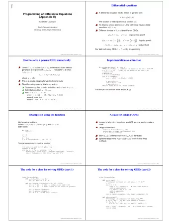
Solving mixed-integer partial differential equation constrained optimization Sven Leyffer 1 , Sebastian Sager 2 , and Anna Th¨ unen 1 , 2 1 Argonne National Laboratory and 2 University of Magdeburg September 1, 2016 1 / 21

Problem Definition and Motivation Approach: First Discretize then Optimize Every Day Problem . . . . . . Control of Heat Equation [Iftime and Demetriou(2009)] Solving MIPDECOs Summary Outlook 2 / 21

Problem Definition and Motivation Motivation: Physics combined with discrete choices, e.g. ◮ Topology optimization ◮ Energy (fossil & renewable) ◮ new problem class ⇒ new approaches u , v , w F ( u , v , w ) min (integrals) s.t. C ( u , v , w ) = 0 (PDE+cond.) u ∈ U , v ∈ V and w ∈ W (function spaces) , e.g. time and space dependency ◮ u ( t , x , y , z ): PDE states ◮ v ( t , x , y , z ): continuous controls ◮ w ( t , x , y , z ): binary (controls) are infinite-dimensional 3 / 21

Approach: First Discretize then Optimize MIPDECO integrals, e.g. Discretize PDE, e.g. finite Objective Constraints trapezoidal rule model differences binaries may high dimensional MINLP depend on discretization Solve! Straight State Rounding forward elimination optimality & slow optimality & fast good & faster 4 / 21

Every Day Problem . . . 5 / 21

. . . Control of Heat Equation [Iftime and Demetriou(2009)] ◮ adapted by Hante ISMP2015 ◮ Control temperature with actuator (= hairdryer) ◮ Select sequence of control inputs (actuators) over time ◮ Continuous control: intensity . . . heat/cool ◮ Match prescribed temperature profile (no fog) ◮ . . . de-fog bathroom mirror with hairdryer 6 / 21

Control of Heat Equation: Mathematical Formulation 9 1 || u ( t f ) || 2 2 , Ω + 2 || u || 2 � || v l || 2 min 2 , Ω × T + objective 2 , T 500 u , v , w l =1 9 ∂ u � s.t. ∂ t − κ ∆ u = in Ω × T heat eq v l f l l =1 u = 0 on ∂ Ω × T Dirichlet u (0) = 100 sin( π x ) sin( π y ) in Ω initial state − Mw l ≤ v l ≤ Mw l for all l ∈ { 1 , . . . , 9 } in T big M 9 � w l = 1 in T source budget l =1 w l ( t ) ∈ { 0 , 1 } for all l ∈ { 1 , . . . , 9 } in T binary . ◮ u ( t , x , y ) states (=temperature) ◮ v l ( t ) continous controls (=intensity) ◮ w l ( t ) binary controls (=location) 7 / 21

How does the solution look like? (Loading HeatAct32Rnd.avi) 8 / 21

Solving MIPDECOs: Straight Forward MINLP ◮ discretize heat equation & other constraints ⇒ MIQP ◮ build a model in AMPL ◮ apply preferred MIQP solver (CPLEX, GUROBI, BONMIN, . . . ) ..easy peasy? Mesh size 8 16 32 64 Variables total 984 7728 63072 513216 binary 72 144 288 576 CPU (CPLEX) 7 . 3 5567 . 3 − − 9 / 21

Solving MIPDECOs: Elimination of PDE 9 ∂ u � ∂ t − κ ∆ u = v l f l l =1 ⇒ AU = BV + d u | ∂ Ω = 0 u (0) = 100 sin( π x ) sin( π y ) ◮ A : 5-point-stencil & implicit euler for heat equation ◮ U = vec( u ): states, dim( U ) = 2 N 2 T n ◮ B : gaussian source term f ◮ V = vec( v ): continous controls, dim( V ) = 9 T n ◮ d : initial/boundary conditions ◮ we add binaries w later to assure that only in one location a hairdryer is operated 10 / 21

Solving MIPDECOs: Elimination of PDE (continued) 9 T n � AU = BV + d ⇔ AU = B V i e i + d i =1 9 T n � A − 1 Be i A − 1 d ⇔ U = + V i � �� � � �� � i =1 homogeneous part inhomogeneous part 1. solve (9 T n + 1) linear systems u hom. ) = A − 1 d and vec(¯ u t , l ) = A − 1 Be i ⇒ vec(¯ 2. solve reduced MIQP: ⇒ v ∗ ◮ no states, 9 T n continous ( v t , l ), 9 T n binary ( w t , l ) ◮ ¯ u data in objective u t , l + ¯ 3. construct the solution: u = v ∗ t , l ¯ u hom. 11 / 21

Solving MIPDECOs: Elimination of PDE (continued) Mesh size 8 16 32 Straight forward CPLEX 7 . 3 5567 . 3 − Elimination total 0 . 4 6 . 3 137 . 5 Linear systems (IPOPT) 0 . 1 3 . 3 123 . 2 MIQP (CPLEX) 0 . 3 2 . 9 14 . 3 Elim. with convolution total 1 . 0 3 . 4 16 . 8 Linear systems (IPOPT) 0 . 0 0 . 2 3 . 6 MIQP (CPLEX) 1 . 0 3 . 2 13 . 2 ◮ optimality ◮ using convolution: only 9 instead of 9 T n linear systems prior to optimization ◮ doesn’t work for nonlinear PDEs, e.g. Helmholtz Eq 12 / 21

Solving MIPDECOs: Sum-Up Rounding ◮ space discretized PDE ⇒ set of ODEs ◮ apply Sum-up Rounding [Sager(2005)] for Optimal Control in every location Integer relaxation of MIQP w t w t ⇒ fractional ( ˜ w 1 , . . . , ˜ w T n ) for 1 every location For t = 1 , . . . , T n ◮ Compute rounding residual: t − 1 0.5 � r t = ˜ w t + ( ˜ w τ − w τ ) τ =0 w t ˜ ◮ Round: � 1 if r t > 1 2 w t = 0 else 0 t 1 2 3 4 5 End 13 / 21

Solving MIPDECOs: Sum-Up Rounding (continued) ◮ do ODE-Sum-up Rounding in every location ◮ Theory for ODE Sum-up Rounding ◮ between proceeding to the next location we may resolve (integer relaxation of remaining sub-MIQP) ◮ doesn’t satisfy the source budget (only one hairdryer) for all 9 � t = 1 , . . . , T n : w t , l = 1 l =1 ◮ how to choose processing order of the locations? ◮ cheap, but large optimality gap Mesh size #QPs 8 16 32 CPU time with resolve 9+1 0 . 03 1 . 74 55 . 86 CPU time without resolve 2 0 . 00 0 . 43 15 . 18 Opt. gap with resolve 9+1 0 . 66 0 . 75 0 . 66 Opt. gap without resolve 2 1 . 03 1 . 37 1 . 23 14 / 21

Solving MIPDECOs: Knapsack-SUR Rounding ◮ SUR cheap, but large optimality gap ◮ Knapsack expensive, but small/no optimality gap ⇒ Combine! For t = 1 , . . . , T n ◮ %choose location largest continous control ¯ l = argmax l | v t , l | (Knapsack Rounding) ◮ calculate rounding residual r t , l ◮ choose location largest residual ¯ l = argmax l | r t , l | ◮ fix w t , ¯ l = 1, all other w t , l = 0 ◮ solve integer relaxation of remaining sub-MIQP (resolve, optional) End 15 / 21

Solving MIPDECOs: Knapsack-SUR Rounding (continued) ◮ combines advantages of Knapsack and SUR Rounding ◮ preserves optimality of Knapsack in the resolved version ◮ reduce optimality gap in simple version Mesh size ( T n ) #QPs 8 16 32 CPU with resolve T n +1 0 . 03 1 . 93 190 . 95 CPU without resolve 2 0 . 01 0 . 23 17 . 27 Opt. gap with resolve T n +1 - - - Opt. gap without resolve 2 < 0 . 01 < 0 . 001 < 0 . 01 16 / 21

Summary Mesh size 8 16 32 #QPs CPU gap CPU gap CPU gap > 10 4 MIQP - 7 . 3 - - - - PDE simple 9 T n LS 0 . 4 - 6 . 3 - 137 . 5 - Elim. convol. 9 LS 1 . 0 - 3 . 4 - 16 . 8 - SUR resolve 9+1 0 . 0 0 . 7 1 . 7 0 . 8 55 . 9 0 . 7 simple 2 0 . 0 1 . 0 0 . 4 1 . 4 15 . 2 1 . 2 Knap- resolve T n +1 0 . 0 - 2 . 5 - 194 . 7 - sack simple 2 0 . 0 0 . 01 0 . 3 0 . 02 15 . 9 0 . 26 Knap. resolve T n +1 0 . 0 - 1 . 9 - 191 . 0 - SUR simple 2 0 . 0 < 0 . 01 0 . 2 < 0 . 001 17 . 3 < 0 . 01 ◮ PDE Elimination works well ◮ Knapsack-SUR as well ◮ Rounding possible even if PDE nonlinear 17 / 21

Outlook ◮ develop theory ◮ move AMPL code to more efficient frameworks ◮ parallelization ◮ more challenging problems, such as nonlinear PDEs Cloaking [Haslinger and M¨ akinen(2015)] (Helmholtz equation) (a) Scatterer (b) u without resolve (c) u with resolve 18 / 21

References I P. Belotti, C. Kirches, S. Leyffer, J. Linderoth, J. Luedtke, and A. Mahajan. Mixed-integer nonlinear optimization. Acta Numerica , 22:1–131, 5 2013. ISSN 1474-0508. J. Haslinger and R. A. M¨ akinen. On a topology optimization problem governed by two-dimensional helmholtz equation. Comput. Optim. Appl. , 62(2):517–544, Nov. 2015. ISSN 0926-6003. O. V. Iftime and M. A. Demetriou. Optimal control of switched distributed parameter systems with spatially scheduled actuators. Automatica , 45(2):312 – 323, 2009. ISSN 0005-1098. 19 / 21

References II S. Sager. Numerical methods for mixed-integer optimal control problems . Der andere Verlag, T¨ onning, L¨ ubeck, Marburg, 2005. ISBN 3-89959-416-9. F. Tr¨ oltzsch. Optimal Control of Partial Differential Equations , volume 112 of Graduate Studies in Mathematics . American Mathematical Society, Providence, 2010. A. W¨ achter and T. L. Biegler. On the implementation of an interior-point filter line-search algorithm for large-scale nonlinear programming. Mathematical Programming , 106(1):25–57, 2006. ISSN 1436-4646. 20 / 21

Pictures https://s-media-cache- ak0.pinimg.com/236x/de/9d/17/de9d1746ab1a644a56f4e81d058a0f44.jpg http://images.travelpod.com/users/lduckett/2.1235847600.anti- fog-mirrorx.jpg https://travelqueentips.files.wordpress.com/2010/02/p2220006.jpg http://sharein.org/wp-content/uploads/2015/10/foggy-mirror- rectify-it-with-petrolium-jelly.jpg https://s-media-cache- ak0.pinimg.com/736x/0c/d3/f5/0cd3f502ce2afaaa2af0e6ab291d4c5b.jpg http://3.bp.blogspot.com/-TcTMQ63GeKQ/UZJYHW- nJGI/AAAAAAAAABE/5Rtke7XS1ug/s1600/PIKACHU-pikachu- 29274386-861-927.jpg http://orig05.deviantart.net/4594/f/2012/200/d/8/pikachu is - happy by otakuron-d57tnmg.png 21 / 21