Soft gluon contributions to Drell-Yan and Higgs productions beyond - - PowerPoint PPT Presentation

• p. 1/24

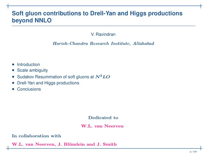
Soft gluon contributions to Drell-Yan and Higgs productions beyond NNLO

• V. Ravindran

Harish-Chandra Research Institute, Allahabad

• Introduction
• Scale ambiguity
• Sudakov Resummation of soft gluons at N3LO
• Drell-Yan and Higgs productions
• Conclusions

Dedicated to W.L. van Neerven In collaboration with W.L. van Neerven, J. Bl¨ umlein and J. Smith

• p. 2/24

Snap shot of the talk

• p. 2/24

Snap shot of the talk

• Perturbative QCD provides a frame work to compute observables at high energies

• p. 2/24

Snap shot of the talk

• Perturbative QCD provides a frame work to compute observables at high energies
• They are "often" sensitive to

1) Renormalisation scale 2) Factorisation scale 3) Non-perturbative quantities that enter 4) Missing higher order contributions(stability of perturbation)

• p. 2/24

Snap shot of the talk

• Perturbative QCD provides a frame work to compute observables at high energies
• They are "often" sensitive to

1) Renormalisation scale 2) Factorisation scale 3) Non-perturbative quantities that enter 4) Missing higher order contributions(stability of perturbation)

• Higher order QCD corrections reduce these effects

• p. 2/24

Snap shot of the talk

• Perturbative QCD provides a frame work to compute observables at high energies
• They are "often" sensitive to

1) Renormalisation scale 2) Factorisation scale 3) Non-perturbative quantities that enter 4) Missing higher order contributions(stability of perturbation)

• Higher order QCD corrections reduce these effects
• Soft gluons dominate in some kinematic regions that are accessible at hadron colliders.

• p. 2/24

Snap shot of the talk

• Perturbative QCD provides a frame work to compute observables at high energies
• They are "often" sensitive to

1) Renormalisation scale 2) Factorisation scale 3) Non-perturbative quantities that enter 4) Missing higher order contributions(stability of perturbation)

• Higher order QCD corrections reduce these effects
• Soft gluons dominate in some kinematic regions that are accessible at hadron colliders.
• Sudakov resummation of soft gluons can be used to predict for Higgs and Drell-Yan total

cross section and rapidity distribution beyond NNLO.

• p. 3/24

Factorisation Theorem (QCD improved Parton Model)

Collins, Soper, Sterman Hadronic cross section in terms of partonic cross sections convoluted with appropriate PDF: 2S dσP1P2 ` τ, m2

h

´ = X

ab

Z 1

τ

dx x Φab (x, µF ) 2ˆ s dˆ σab “τ x, m2

h, µF

”

• p. 3/24

Factorisation Theorem (QCD improved Parton Model)

Collins, Soper, Sterman Hadronic cross section in terms of partonic cross sections convoluted with appropriate PDF: 2S dσP1P2 ` τ, m2

h

´ = X

ab

Z 1

τ

dx x Φab (x, µF ) 2ˆ s dˆ σab “τ x, m2

h, µF

”

• The perturbatively calculable partonic cross section:

dˆ σab `z, m2

h, µF

´ =

∞

X

i=0

„ αs(µR) 4π «i dˆ σab,(i) `z, m2

h, µF , µR

´

• p. 3/24

Factorisation Theorem (QCD improved Parton Model)

Collins, Soper, Sterman Hadronic cross section in terms of partonic cross sections convoluted with appropriate PDF: 2S dσP1P2 ` τ, m2

h

´ = X

ab

Z 1

τ

dx x Φab (x, µF ) 2ˆ s dˆ σab “τ x, m2

h, µF

”

• The perturbatively calculable partonic cross section:

dˆ σab `z, m2

h, µF

´ =

∞

X

i=0

„ αs(µR) 4π «i dˆ σab,(i) `z, m2

h, µF , µR

´

• The non-perturbative flux:

Φab(x, µF ) = Z 1

x

dz z fa (z, µF ) fb “x z , µF ”

• p. 3/24

Factorisation Theorem (QCD improved Parton Model)

Collins, Soper, Sterman Hadronic cross section in terms of partonic cross sections convoluted with appropriate PDF: 2S dσP1P2 ` τ, m2

h

´ = X

ab

Z 1

τ

dx x Φab (x, µF ) 2ˆ s dˆ σab “τ x, m2

h, µF

”

• The perturbatively calculable partonic cross section:

dˆ σab `z, m2

h, µF

´ =

∞

X

i=0

„ αs(µR) 4π «i dˆ σab,(i) `z, m2

h, µF , µR

´

• The non-perturbative flux:

Φab(x, µF ) = Z 1

x

dz z fa (z, µF ) fb “x z , µF ”

• fP1

a

(x, µF ) are Parton distribution functions with momentum fraction x.

• p. 3/24

Factorisation Theorem (QCD improved Parton Model)

Collins, Soper, Sterman Hadronic cross section in terms of partonic cross sections convoluted with appropriate PDF: 2S dσP1P2 ` τ, m2

h

´ = X

ab

Z 1

τ

dx x Φab (x, µF ) 2ˆ s dˆ σab “τ x, m2

h, µF

”

• The perturbatively calculable partonic cross section:

dˆ σab `z, m2

h, µF

´ =

∞

X

i=0

„ αs(µR) 4π «i dˆ σab,(i) `z, m2

h, µF , µR

´

• The non-perturbative flux:

Φab(x, µF ) = Z 1

x

dz z fa (z, µF ) fb “x z , µF ”

• fP1

a

(x, µF ) are Parton distribution functions with momentum fraction x.

• µR is the Renormalisation scale and µF , Factorisation scale

• p. 3/24

Factorisation Theorem (QCD improved Parton Model)

Collins, Soper, Sterman Hadronic cross section in terms of partonic cross sections convoluted with appropriate PDF: 2S dσP1P2 ` τ, m2

h

´ = X

ab

Z 1

τ

dx x Φab (x, µF ) 2ˆ s dˆ σab “τ x, m2

h, µF

”

• The perturbatively calculable partonic cross section:

dˆ σab `z, m2

h, µF

´ =

∞

X

i=0

„ αs(µR) 4π «i dˆ σab,(i) `z, m2

h, µF , µR

´

• The non-perturbative flux:

Φab(x, µF ) = Z 1

x

dz z fa (z, µF ) fb “x z , µF ”

• fP1

a

(x, µF ) are Parton distribution functions with momentum fraction x.

• µR is the Renormalisation scale and µF , Factorisation scale
• The Renormalisation group invariance:

d dµ σP1P2(τ, m2 h) = 0,

µ = µF , µR

• p. 4/24

Higgs production at LHC and Scale dependence

Harlander, Kilgore/ Anastasiou, Melnikov/ van Neerven, Smith, VR

• p. 4/24

Higgs production at LHC and Scale dependence

Harlander, Kilgore/ Anastasiou, Melnikov/ van Neerven, Smith, VR

1 10 100 120 140 160 180 200 220 240 260 280 300 σ(pp→H+X) [pb] MH [GeV] LO Harlander NLO NNLO √ s = 14 TeV

• p. 4/24

Higgs production at LHC and Scale dependence

Harlander, Kilgore/ Anastasiou, Melnikov/ van Neerven, Smith, VR

1 10 100 120 140 160 180 200 220 240 260 280 300 σ(pp→H+X) [pb] MH [GeV] LO Harlander NLO NNLO √ s = 14 TeV

0.1 1 10

µ/µ

0.4 0.6 0.8 1 1.2 1.4 1.6 1.8 2 2.2

N

LO NLO NNLO

• See Hinchcliff,... for LO and see Dawson, Djouadi et.al for NLO (with finite top mass), NNLO

is done in the large top limit N = σ(µR = µF = µ)/σ(µ0).

• p. 4/24

Higgs production at LHC and Scale dependence

Harlander, Kilgore/ Anastasiou, Melnikov/ van Neerven, Smith, VR

1 10 100 120 140 160 180 200 220 240 260 280 300 σ(pp→H+X) [pb] MH [GeV] LO Harlander NLO NNLO √ s = 14 TeV

0.1 1 10

µ/µ

0.4 0.6 0.8 1 1.2 1.4 1.6 1.8 2 2.2

N

LO NLO NNLO

• See Hinchcliff,... for LO and see Dawson, Djouadi et.al for NLO (with finite top mass), NNLO

is done in the large top limit N = σ(µR = µF = µ)/σ(µ0).

• Is it the end?

• p. 5/24

Soft part of NNLO

Catani et al, Harlander and Kilgore

• p. 5/24

Soft part of NNLO

Catani et al, Harlander and Kilgore 2S dσP1P2 (τ, mh) = X

ab

Z 1

τ

dx x Φab (x) 2ˆ s dˆ σab “τ x, mh ” τ = m2

h

S

10 100 1000 10000 100000 1e+06 1e+07 0.001 0.002 0.003 0.004 0.005 0.006

φab

x = Q2/S

LHC ( S = (14 TeV)^2)

qqb gg

(0.01)qg

Gluon flux is largest at LHC

• p. 5/24

Soft part of NNLO

Catani et al, Harlander and Kilgore 2S dσP1P2 (τ, mh) = X

ab

Z 1

τ

dx x Φab (x) 2ˆ s dˆ σab “τ x, mh ” τ = m2

h

S

10 100 1000 10000 100000 1e+06 1e+07 0.001 0.002 0.003 0.004 0.005 0.006

φab

x = Q2/S

LHC ( S = (14 TeV)^2)

qqb gg

(0.01)qg

Gluon flux is largest at LHC

• Φab(x) becomes large when

x → xmin = τ

• p. 5/24

Soft part of NNLO

Catani et al, Harlander and Kilgore 2S dσP1P2 (τ, mh) = X

ab

Z 1

τ

dx x Φab (x) 2ˆ s dˆ σab “τ x, mh ” τ = m2

h

S

10 100 1000 10000 100000 1e+06 1e+07 0.001 0.002 0.003 0.004 0.005 0.006

φab

x = Q2/S

LHC ( S = (14 TeV)^2)

qqb gg

(0.01)qg

Gluon flux is largest at LHC

• Φab(x) becomes large when

x → xmin = τ

• Dominant contribution to Higgs production

comes from the region when x → τ

• p. 5/24

Soft part of NNLO

Catani et al, Harlander and Kilgore 2S dσP1P2 (τ, mh) = X

ab

Z 1

τ

dx x Φab (x) 2ˆ s dˆ σab “τ x, mh ” τ = m2

h

S

10 100 1000 10000 100000 1e+06 1e+07 0.001 0.002 0.003 0.004 0.005 0.006

φab

x = Q2/S

LHC ( S = (14 TeV)^2)

qqb gg

(0.01)qg

Gluon flux is largest at LHC

• Φab(x) becomes large when

x → xmin = τ

• Dominant contribution to Higgs production

comes from the region when x → τ

• It is sufficient if we know the partonic cross

section when x → τ

• p. 5/24

Soft part of NNLO

Catani et al, Harlander and Kilgore 2S dσP1P2 (τ, mh) = X

ab

Z 1

τ

dx x Φab (x) 2ˆ s dˆ σab “τ x, mh ” τ = m2

h

S

10 100 1000 10000 100000 1e+06 1e+07 0.001 0.002 0.003 0.004 0.005 0.006

φab

x = Q2/S

LHC ( S = (14 TeV)^2)

qqb gg

(0.01)qg

Gluon flux is largest at LHC

• Φab(x) becomes large when

x → xmin = τ

• Dominant contribution to Higgs production

comes from the region when x → τ

• It is sufficient if we know the partonic cross

section when x → τ

• x → τ is called soft limit.

• p. 5/24

Soft part of NNLO

Catani et al, Harlander and Kilgore 2S dσP1P2 (τ, mh) = X

ab

Z 1

τ

dx x Φab (x) 2ˆ s dˆ σab “τ x, mh ” τ = m2

h

S

10 100 1000 10000 100000 1e+06 1e+07 0.001 0.002 0.003 0.004 0.005 0.006

φab

x = Q2/S

LHC ( S = (14 TeV)^2)

qqb gg

(0.01)qg

Gluon flux is largest at LHC

• Φab(x) becomes large when

x → xmin = τ

• Dominant contribution to Higgs production

comes from the region when x → τ

• It is sufficient if we know the partonic cross

section when x → τ

• x → τ is called soft limit.
• Expand the partonic cross section around

x = τ.

• p. 6/24

Soft part

Catani et al, Harlander and Kilgore

• p. 6/24

Soft part

Catani et al, Harlander and Kilgore

• Expand the partonic cross section around x = τ or z = x

τ = 1.

• p. 6/24

Soft part

Catani et al, Harlander and Kilgore

• Expand the partonic cross section around x = τ or z = x

τ = 1.

dˆ σ(z) = C(0)(z) +

∞

X

i=1

(1 − z)iC(i) z = x τ

• p. 6/24

Soft part

Catani et al, Harlander and Kilgore

• Expand the partonic cross section around x = τ or z = x

τ = 1.

dˆ σ(z) = C(0)(z) +

∞

X

i=1

(1 − z)iC(i) z = x τ

• C(0):

C(0) = C(0) δ(1 − z) +

∞

X

k=0

C(k) logk(1 − z) (1 − z) !

+

• p. 6/24

Soft part

Catani et al, Harlander and Kilgore

• Expand the partonic cross section around x = τ or z = x

τ = 1.

dˆ σ(z) = C(0)(z) +

∞

X

i=1

(1 − z)iC(i) z = x τ

• C(0):

C(0) = C(0) δ(1 − z) +

∞

X

k=0

C(k) logk(1 − z) (1 − z) !

+

• C(i)

will be pure constants such as ζ(2), ζ(3).

• p. 6/24

Soft part

Catani et al, Harlander and Kilgore

• Expand the partonic cross section around x = τ or z = x

τ = 1.

dˆ σ(z) = C(0)(z) +

∞

X

i=1

(1 − z)iC(i) z = x τ

• C(0):

C(0) = C(0) δ(1 − z) +

∞

X

k=0

C(k) logk(1 − z) (1 − z) !

+

• C(i)

will be pure constants such as ζ(2), ζ(3).

• Compute the entire cross section in the "soft limit".

• p. 6/24

Soft part

Catani et al, Harlander and Kilgore

• Expand the partonic cross section around x = τ or z = x

τ = 1.

dˆ σ(z) = C(0)(z) +

∞

X

i=1

(1 − z)iC(i) z = x τ

• C(0):

C(0) = C(0) δ(1 − z) +

∞

X

k=0

C(k) logk(1 − z) (1 − z) !

+

• C(i)

will be pure constants such as ζ(2), ζ(3).

• Compute the entire cross section in the "soft limit".

OR Extract from "Form factors and DGLAP kernels" using 1) Factorisation theorem 2) Renormalisation Group Invariance 3) Drell-Yan NNLO results

• p. 7/24

Soft plus Virtual at N 3LO and beyond

VR

• p. 7/24

Soft plus Virtual at N 3LO and beyond

VR Using "factorisation" of Virtual, Soft and Collinear: ∆sv

I,P (z, q2, µ2 R, µ2 F ) = C exp

ΨI

P (z, q2, µ2 R, µ2 F , ε)

!˛ ˛ ˛ ˛ ˛

ε=0

I = q, g n = 4 + ε

• p. 7/24

Soft plus Virtual at N 3LO and beyond

VR Using "factorisation" of Virtual, Soft and Collinear: ∆sv

I,P (z, q2, µ2 R, µ2 F ) = C exp

ΨI

P (z, q2, µ2 R, µ2 F , ε)

!˛ ˛ ˛ ˛ ˛

ε=0

I = q, g n = 4 + ε ΨI

P (z, q2, µ2 R, µ2 F , ε)

= ln “ ZI (ˆ as, µ2

R, µ2, ε)

”2 + ln ˛ ˛ ˆ F I(ˆ as, Q2, µ2, ε) ˛ ˛2 ! δ(1 − z) +2 Φ I

P (ˆ

as, q2, µ2, z, ε) − 2 m C ln ΓII(ˆ as, µ2, µ2

F , z, ε)

• p. 7/24

Soft plus Virtual at N 3LO and beyond

VR Using "factorisation" of Virtual, Soft and Collinear: ∆sv

I,P (z, q2, µ2 R, µ2 F ) = C exp

ΨI

P (z, q2, µ2 R, µ2 F , ε)

!˛ ˛ ˛ ˛ ˛

ε=0

I = q, g n = 4 + ε ΨI

P (z, q2, µ2 R, µ2 F , ε)

= ln “ ZI (ˆ as, µ2

R, µ2, ε)

”2 + ln ˛ ˛ ˆ F I(ˆ as, Q2, µ2, ε) ˛ ˛2 ! δ(1 − z) +2 Φ I

P (ˆ

as, q2, µ2, z, ε) − 2 m C ln ΓII(ˆ as, µ2, µ2

F , z, ε)

• ZI(ˆ

as, µ2

R, µ2, ε) is operator renormalisation constant with µ is mass parameter in

n = 4 + ε dimensional regularisation → N3LO

• ˆ

F I(ˆ as, Q2, µ2, ε) is the Form factor with Q2 = −q2 → N3LO

• Φ I

P (ˆ

as, q2, µ2, z, ε) is the soft distribution function → NNLO level

• ΓII(ˆ

as, µ2, µ2

F , z, ε) is mass factorisation kernel → N3LO

• p. 7/24

Soft plus Virtual at N 3LO and beyond

VR Using "factorisation" of Virtual, Soft and Collinear: ∆sv

I,P (z, q2, µ2 R, µ2 F ) = C exp

ΨI

P (z, q2, µ2 R, µ2 F , ε)

!˛ ˛ ˛ ˛ ˛

ε=0

I = q, g n = 4 + ε ΨI

P (z, q2, µ2 R, µ2 F , ε)

= ln “ ZI (ˆ as, µ2

R, µ2, ε)

”2 + ln ˛ ˛ ˆ F I(ˆ as, Q2, µ2, ε) ˛ ˛2 ! δ(1 − z) +2 Φ I

P (ˆ

as, q2, µ2, z, ε) − 2 m C ln ΓII(ˆ as, µ2, µ2

F , z, ε)

• ZI(ˆ

as, µ2

R, µ2, ε) is operator renormalisation constant with µ is mass parameter in

n = 4 + ε dimensional regularisation → N3LO

• ˆ

F I(ˆ as, Q2, µ2, ε) is the Form factor with Q2 = −q2 → N3LO

• Φ I

P (ˆ

as, q2, µ2, z, ε) is the soft distribution function → NNLO level

• ΓII(ˆ

as, µ2, µ2

F , z, ε) is mass factorisation kernel → N3LO

ˆ as = ˆ g2

s

16π2 m = 1 2 for DIS, m = 1 for DY, Higgs

• p. 8/24

Sudakov Resummation for Form factors

Vogt,Vermaseren,Moch,VR

• p. 8/24

Sudakov Resummation for Form factors

Vogt,Vermaseren,Moch,VR Q2 d dQ2 ln ˆ F I ` ˆ as, Q2, µ2, ε ´ = 1 2 " KI ˆ as, µ2

R

µ2 , ε ! + GI ˆ as, Q2 µ2

R

, µ2

R

µ2 , ε ! # Solution : ln ˆ F I(ˆ as, Q2, µ2, ε) =

∞

X

i=1

ˆ ai

s

„Q2 µ2 «i ε

2

Si

ε ˆ

LI,(i)

F

(ε)

• p. 8/24

Sudakov Resummation for Form factors

Vogt,Vermaseren,Moch,VR Q2 d dQ2 ln ˆ F I ` ˆ as, Q2, µ2, ε ´ = 1 2 " KI ˆ as, µ2

R

µ2 , ε ! + GI ˆ as, Q2 µ2

R

, µ2

R

µ2 , ε ! # Solution : ln ˆ F I(ˆ as, Q2, µ2, ε) =

∞

X

i=1

ˆ ai

s

„Q2 µ2 «i ε

2

Si

ε ˆ

LI,(i)

F

(ε) Formal solution upto 4 loops: ˆ LI,(1)

F

= 1 ε2 − 2AI

1

! + 1 ε GI

1(ε)

! ˆ LI,(2)

F

= 1 ε3 β0AI

1

! + 1 ε2 − 1 2AI

2 − β0GI 1(ε)

! + 1 2εGI

2(ε)

· · · · · · · · · · · · · · · · · · · · · · · · · · · · · · ··

• p. 8/24

Sudakov Resummation for Form factors

Vogt,Vermaseren,Moch,VR Q2 d dQ2 ln ˆ F I ` ˆ as, Q2, µ2, ε ´ = 1 2 " KI ˆ as, µ2

R

µ2 , ε ! + GI ˆ as, Q2 µ2

R

, µ2

R

µ2 , ε ! # Solution : ln ˆ F I(ˆ as, Q2, µ2, ε) =

∞

X

i=1

ˆ ai

s

„Q2 µ2 «i ε

2

Si

ε ˆ

LI,(i)

F

(ε) Formal solution upto 4 loops: ˆ LI,(1)

F

= 1 ε2 − 2AI

1

! + 1 ε GI

1(ε)

! ˆ LI,(2)

F

= 1 ε3 β0AI

1

! + 1 ε2 − 1 2AI

2 − β0GI 1(ε)

! + 1 2εGI

2(ε)

· · · · · · · · · · · · · · · · · · · · · · · · · · · · · · ··

• AI

are maximally non − abelian Ag

i = CA

CF Aq

i

i = 1, 2, 3.

• p. 8/24

Sudakov Resummation for Form factors

Vogt,Vermaseren,Moch,VR Q2 d dQ2 ln ˆ F I ` ˆ as, Q2, µ2, ε ´ = 1 2 " KI ˆ as, µ2

R

µ2 , ε ! + GI ˆ as, Q2 µ2

R

, µ2

R

µ2 , ε ! # Solution : ln ˆ F I(ˆ as, Q2, µ2, ε) =

∞

X

i=1

ˆ ai

s

„Q2 µ2 «i ε

2

Si

ε ˆ

LI,(i)

F

(ε) Formal solution upto 4 loops: ˆ LI,(1)

F

= 1 ε2 − 2AI

1

! + 1 ε GI

1(ε)

! ˆ LI,(2)

F

= 1 ε3 β0AI

1

! + 1 ε2 − 1 2AI

2 − β0GI 1(ε)

! + 1 2εGI

2(ε)

· · · · · · · · · · · · · · · · · · · · · · · · · · · · · · ··

• AI

are maximally non − abelian Ag

i = CA

CF Aq

i

i = 1, 2, 3.

• Every order in ˆ

as, all the poles except the lowest one can be predicted from the previous

• rder results using A and β function.

• p. 9/24

New observation for single pole in ε

VR,Smith,van Neerven

• p. 9/24

New observation for single pole in ε

VR,Smith,van Neerven Two loop results for ˆ F q and ˆ F g in SU(N) solves the single pole problem:

• p. 9/24

New observation for single pole in ε

VR,Smith,van Neerven Two loop results for ˆ F q and ˆ F g in SU(N) solves the single pole problem: GIs have interesting structure: GI

1(ε)

= 2(BI

1 − γI 1) + fI 1 + ∞

X

k=1

εkg I,k

1

GI

2(ε)

= 2(BI

2 − γI 2) + fI 2 − 2β0g I,1 1

+

∞

X

k=1

εkg I,k

2

• p. 9/24

New observation for single pole in ε

VR,Smith,van Neerven Two loop results for ˆ F q and ˆ F g in SU(N) solves the single pole problem: GIs have interesting structure: GI

1(ε)

= 2(BI

1 − γI 1) + fI 1 + ∞

X

k=1

εkg I,k

1

GI

2(ε)

= 2(BI

2 − γI 2) + fI 2 − 2β0g I,1 1

+

∞

X

k=1

εkg I,k

2

BI

i are δ(1 − z) part of PII splitting functions. The new constants "fI 1 and fI 2 " satisfy

fg

i = CA

CF fq

i

i = 1, 2

• p. 9/24

New observation for single pole in ε

VR,Smith,van Neerven Two loop results for ˆ F q and ˆ F g in SU(N) solves the single pole problem: GIs have interesting structure: GI

1(ε)

= 2(BI

1 − γI 1) + fI 1 + ∞

X

k=1

εkg I,k

1

GI

2(ε)

= 2(BI

2 − γI 2) + fI 2 − 2β0g I,1 1

+

∞

X

k=1

εkg I,k

2

BI

i are δ(1 − z) part of PII splitting functions. The new constants "fI 1 and fI 2 " satisfy

fg

i = CA

CF fq

i

i = 1, 2 Even the single pole can be predicted: GI

i = 2(BI i − γI i ) + fI i + · · ·

• p. 9/24

New observation for single pole in ε

VR,Smith,van Neerven Two loop results for ˆ F q and ˆ F g in SU(N) solves the single pole problem: GIs have interesting structure: GI

1(ε)

= 2(BI

1 − γI 1) + fI 1 + ∞

X

k=1

εkg I,k

1

GI

2(ε)

= 2(BI

2 − γI 2) + fI 2 − 2β0g I,1 1

+

∞

X

k=1

εkg I,k

2

BI

i are δ(1 − z) part of PII splitting functions. The new constants "fI 1 and fI 2 " satisfy

fg

i = CA

CF fq

i

i = 1, 2 Even the single pole can be predicted: GI

i = 2(BI i − γI i ) + fI i + · · ·

Recent three loop result by Moch,Vermaseren, Vogt confirms our prediction: fg

3 = CA

CF fq

3

• p. 9/24

New observation for single pole in ε

VR,Smith,van Neerven Two loop results for ˆ F q and ˆ F g in SU(N) solves the single pole problem: GIs have interesting structure: GI

1(ε)

= 2(BI

1 − γI 1) + fI 1 + ∞

X

k=1

εkg I,k

1

GI

2(ε)

= 2(BI

2 − γI 2) + fI 2 − 2β0g I,1 1

+

∞

X

k=1

εkg I,k

2

BI

i are δ(1 − z) part of PII splitting functions. The new constants "fI 1 and fI 2 " satisfy

fg

i = CA

CF fq

i

i = 1, 2 Even the single pole can be predicted: GI

i = 2(BI i − γI i ) + fI i + · · ·

Recent three loop result by Moch,Vermaseren, Vogt confirms our prediction: fg

3 = CA

CF fq

3

This completes the understanding of all the poles of the form factors.

• p. 10/24

Mass factorisation using DGLAP kernel

VR

• p. 10/24

Mass factorisation using DGLAP kernel

VR Due to the massless partons, collinear singularities appear in

• the phase space of the real emission processes
• loop integrals of the virtual corrections

• p. 10/24

Mass factorisation using DGLAP kernel

VR Due to the massless partons, collinear singularities appear in

• the phase space of the real emission processes
• loop integrals of the virtual corrections

They are removed by Mass Factorisation by adding: − ln Γ(ˆ as, µ2, µ2

F , z, ε)

• p. 10/24

Mass factorisation using DGLAP kernel

VR Due to the massless partons, collinear singularities appear in

• the phase space of the real emission processes
• loop integrals of the virtual corrections

They are removed by Mass Factorisation by adding: − ln Γ(ˆ as, µ2, µ2

F , z, ε)

DGLAP kernels satisfy Renormalisation Group Equations: µ2

F

d dµ2

F

Γ(z, µ2

F , ε) = 1

2P ` z, µ2

F

´ ⊗ Γ ` z, µ2

F , ε

´ .

• p. 10/24

Mass factorisation using DGLAP kernel

VR Due to the massless partons, collinear singularities appear in

• the phase space of the real emission processes
• loop integrals of the virtual corrections

They are removed by Mass Factorisation by adding: − ln Γ(ˆ as, µ2, µ2

F , z, ε)

DGLAP kernels satisfy Renormalisation Group Equations: µ2

F

d dµ2

F

Γ(z, µ2

F , ε) = 1

2P ` z, µ2

F

´ ⊗ Γ ` z, µ2

F , ε

´ . The diagonal terms of the splitting functions P (i)(z) have the following structure P (i)

II (z) = 2

" BI

i+1δ(1 − z) + AI i+1D0

# + P (i)

reg,II(z) ,

• p. 10/24

Mass factorisation using DGLAP kernel

VR Due to the massless partons, collinear singularities appear in

• the phase space of the real emission processes
• loop integrals of the virtual corrections

They are removed by Mass Factorisation by adding: − ln Γ(ˆ as, µ2, µ2

F , z, ε)

DGLAP kernels satisfy Renormalisation Group Equations: µ2

F

d dµ2

F

Γ(z, µ2

F , ε) = 1

2P ` z, µ2

F

´ ⊗ Γ ` z, µ2

F , ε

´ . The diagonal terms of the splitting functions P (i)(z) have the following structure P (i)

II (z) = 2

" BI

i+1δ(1 − z) + AI i+1D0

# + P (i)

reg,II(z) ,

D0 = „ 1 1 − z «

+

, P (i)

reg,IIare

regular when z → 1. We will be left with only maximally non-abelian constants AI

i and fI i

• p. 11/24

Finiteness of the Cross section

VR

• p. 11/24

Finiteness of the Cross section

VR Observable ∆I(αs, Q2) are finite: Infra − red safe

• p. 11/24

Finiteness of the Cross section

VR Observable ∆I(αs, Q2) are finite: Infra − red safe The remaining poles after UV Operator Renormalisation(Zαs and ZI) and Mass factorisation: 1 εi+1 at ithloop Highest poles are not removed by renormalisation and factorisation

• p. 11/24

Finiteness of the Cross section

VR Observable ∆I(αs, Q2) are finite: Infra − red safe The remaining poles after UV Operator Renormalisation(Zαs and ZI) and Mass factorisation: 1 εi+1 at ithloop Highest poles are not removed by renormalisation and factorisation

• The structure of soft part should be "similar" to the Form Factors.
• Hence using gauge invariance and RG invariance, we can propose

q2 d dq2 ΦI `ˆ as, q2, µ2, z, ε´ = 1 2 " KI ˆ as, µ2

R

µ2 , z, ε ! + GI ˆ as, q2 µ2

R

, µ2

R

µ2 , z, ε ! #

• p. 11/24

Finiteness of the Cross section

VR Observable ∆I(αs, Q2) are finite: Infra − red safe The remaining poles after UV Operator Renormalisation(Zαs and ZI) and Mass factorisation: 1 εi+1 at ithloop Highest poles are not removed by renormalisation and factorisation

• The structure of soft part should be "similar" to the Form Factors.
• Hence using gauge invariance and RG invariance, we can propose

q2 d dq2 ΦI `ˆ as, q2, µ2, z, ε´ = 1 2 " KI ˆ as, µ2

R

µ2 , z, ε ! + GI ˆ as, q2 µ2

R

, µ2

R

µ2 , z, ε ! # RG invariance of ΦI implies: µ2

R

d dµ2

R

KI ˆ as, µ2

R

µ2 , z, ε ! = −µ2

R

d dµ2

R

GI ˆ as, q2 µ2

R

, µ2

R

µ2 , z, ε ! = −AI(as(µ2

R))δ(1 − z)

• p. 12/24

Solution to (Soft)Sudakov Equation

VR

• p. 12/24

Solution to (Soft)Sudakov Equation

VR Infra-red safeness of the cross section implies A

I = −AI

• p. 12/24

Solution to (Soft)Sudakov Equation

VR Infra-red safeness of the cross section implies A

I = −AI

Solution to (soft) Sudakov equation: ΦI ` ˆ as, q2, µ2, z, ε ´ =

∞

X

i=1

ˆ ai

s

„ q2 µ2 «i ε

2

Si

ε ˆ

ΦI,(i)(z, ε)

• p. 12/24

Solution to (Soft)Sudakov Equation

VR Infra-red safeness of the cross section implies A

I = −AI

Solution to (soft) Sudakov equation: ΦI ` ˆ as, q2, µ2, z, ε ´ =

∞

X

i=1

ˆ ai

s

„ q2 µ2 «i ε

2

Si

ε ˆ

ΦI,(i)(z, ε) where ˆ ΦI,(i)(z, ε) = ˆ LI,(i)

F

(ε) AI → −δ(1 − z) AI, GI(ε) → G I (z, ε) !

• p. 12/24

Solution to (Soft)Sudakov Equation

VR Infra-red safeness of the cross section implies A

I = −AI

Solution to (soft) Sudakov equation: ΦI ` ˆ as, q2, µ2, z, ε ´ =

∞

X

i=1

ˆ ai

s

„ q2 µ2 «i ε

2

Si

ε ˆ

ΦI,(i)(z, ε) where ˆ ΦI,(i)(z, ε) = ˆ LI,(i)

F

(ε) AI → −δ(1 − z) AI, GI(ε) → G I (z, ε) ! Most general solution: ΦI(ˆ as, q2, µ2, z, ε) = ΦI(ˆ as, q2(1 − z)2m, µ2, ε) =

∞

X

i=1

ˆ ai

s

„ q2(1 − z)2m µ2 «i ε

2

Si

ε

„ i m ε 2(1 − z) « ˆ φ I,(i)(ε)

• p. 12/24

Solution to (Soft)Sudakov Equation

VR Infra-red safeness of the cross section implies A

I = −AI

Solution to (soft) Sudakov equation: ΦI ` ˆ as, q2, µ2, z, ε ´ =

∞

X

i=1

ˆ ai

s

„ q2 µ2 «i ε

2

Si

ε ˆ

ΦI,(i)(z, ε) where ˆ ΦI,(i)(z, ε) = ˆ LI,(i)

F

(ε) AI → −δ(1 − z) AI, GI(ε) → G I (z, ε) ! Most general solution: ΦI(ˆ as, q2, µ2, z, ε) = ΦI(ˆ as, q2(1 − z)2m, µ2, ε) =

∞

X

i=1

ˆ ai

s

„ q2(1 − z)2m µ2 «i ε

2

Si

ε

„ i m ε 2(1 − z) « ˆ φ I,(i)(ε) All the poles in ε are predictable.

• p. 13/24

Universal Soft part

VR

• p. 13/24

Universal Soft part

VR Single pole in ε: G

I 1 (ε)

= −fI

1 + ∞

X

k=1

εkG

I,(k) 1

G

I 2 (ε)

= −fI

2 − 2β0G I,(1) 1

+

∞

X

k=1

εkG

I,(k) 2

· · · · · · · · · · · · · · · · · ·

• p. 13/24

Universal Soft part

VR Single pole in ε: G

I 1 (ε)

= −fI

1 + ∞

X

k=1

εkG

I,(k) 1

G

I 2 (ε)

= −fI

2 − 2β0G I,(1) 1

+

∞

X

k=1

εkG

I,(k) 2

· · · · · · · · · · · · · · · · · · Maximally non-abelian: G

g i (ε) = CA

CF G

q i (ε)

i = 1, 2, 3

• p. 13/24

Universal Soft part

VR Single pole in ε: G

I 1 (ε)

= −fI

1 + ∞

X

k=1

εkG

I,(k) 1

G

I 2 (ε)

= −fI

2 − 2β0G I,(1) 1

+

∞

X

k=1

εkG

I,(k) 2

· · · · · · · · · · · · · · · · · · Maximally non-abelian: G

g i (ε) = CA

CF G

q i (ε)

i = 1, 2, 3 Soft part of the any cross section are independent of spin,colour,flavour or other quantum numbers.

• p. 13/24

Universal Soft part

VR Single pole in ε: G

I 1 (ε)

= −fI

1 + ∞

X

k=1

εkG

I,(k) 1

G

I 2 (ε)

= −fI

2 − 2β0G I,(1) 1

+

∞

X

k=1

εkG

I,(k) 2

· · · · · · · · · · · · · · · · · · Maximally non-abelian: G

g i (ε) = CA

CF G

q i (ε)

i = 1, 2, 3 Soft part of the any cross section are independent of spin,colour,flavour or other quantum numbers. Φq(ˆ as, q2, z, µ2, ε) = CF CA Φg(ˆ as, q2, z, µ2, ε)

• p. 14/24

Higgs productions from Drell-Yan beyond NNLO

Universal soft function: VR

• p. 14/24

Higgs productions from Drell-Yan beyond NNLO

Universal soft function: VR Φg(ˆ as, q2, z, µ2, ε) = CA CF Φq(ˆ as, q2, z, µ2, ε)

• From Drell-Yan Φq(ˆ

as, q2, z, ε), Gluon form factor Fg and operator renormalisation constant Zg and DGLAP kernel Γgg, we can compute soft plus virtual part of σ(g + g → Higgs) without explicitly calculating the soft part of Higgs production.

• p. 14/24

Higgs productions from Drell-Yan beyond NNLO

Universal soft function: VR Φg(ˆ as, q2, z, µ2, ε) = CA CF Φq(ˆ as, q2, z, µ2, ε)

• From Drell-Yan Φq(ˆ

as, q2, z, ε), Gluon form factor Fg and operator renormalisation constant Zg and DGLAP kernel Γgg, we can compute soft plus virtual part of σ(g + g → Higgs) without explicitly calculating the soft part of Higgs production.

• Our NNLO predictions agrees with the results by Catani et al, Harlander and Kilgore. No

need for explicit computation of soft contributions for the Higgs production.

• p. 14/24

Higgs productions from Drell-Yan beyond NNLO

Universal soft function: VR Φg(ˆ as, q2, z, µ2, ε) = CA CF Φq(ˆ as, q2, z, µ2, ε)

• From Drell-Yan Φq(ˆ

as, q2, z, ε), Gluon form factor Fg and operator renormalisation constant Zg and DGLAP kernel Γgg, we can compute soft plus virtual part of σ(g + g → Higgs) without explicitly calculating the soft part of Higgs production.

• Our NNLO predictions agrees with the results by Catani et al, Harlander and Kilgore. No

need for explicit computation of soft contributions for the Higgs production.

• Our N3LO predictions (without δ(1 − z) part) for soft plus virtual contributions to Drell-Yan

and Higgs productions agree with the results of Moch and Vogt

• p. 14/24

Higgs productions from Drell-Yan beyond NNLO

Universal soft function: VR Φg(ˆ as, q2, z, µ2, ε) = CA CF Φq(ˆ as, q2, z, µ2, ε)

• From Drell-Yan Φq(ˆ

as, q2, z, ε), Gluon form factor Fg and operator renormalisation constant Zg and DGLAP kernel Γgg, we can compute soft plus virtual part of σ(g + g → Higgs) without explicitly calculating the soft part of Higgs production.

• Our NNLO predictions agrees with the results by Catani et al, Harlander and Kilgore. No

need for explicit computation of soft contributions for the Higgs production.

• Our N3LO predictions (without δ(1 − z) part) for soft plus virtual contributions to Drell-Yan

and Higgs productions agree with the results of Moch and Vogt

• The scalar form factor FS =< P|ψψ|P > can be predicted at three loop from the known

three loop Ai, Bi, fi and γm

i .

• p. 14/24

Higgs productions from Drell-Yan beyond NNLO

Universal soft function: VR Φg(ˆ as, q2, z, µ2, ε) = CA CF Φq(ˆ as, q2, z, µ2, ε)

• From Drell-Yan Φq(ˆ

as, q2, z, ε), Gluon form factor Fg and operator renormalisation constant Zg and DGLAP kernel Γgg, we can compute soft plus virtual part of σ(g + g → Higgs) without explicitly calculating the soft part of Higgs production.

• Our NNLO predictions agrees with the results by Catani et al, Harlander and Kilgore. No

need for explicit computation of soft contributions for the Higgs production.

• Our N3LO predictions (without δ(1 − z) part) for soft plus virtual contributions to Drell-Yan

and Higgs productions agree with the results of Moch and Vogt

• The scalar form factor FS =< P|ψψ|P > can be predicted at three loop from the known

three loop Ai, Bi, fi and γm

i .

• Soft plus Virtual part Higgs production through bottom quark fusion

σ(b + b → Higgs) can be predicted upto N3LO(without δ(1 − z)).

• p. 14/24

Higgs productions from Drell-Yan beyond NNLO

Universal soft function: VR Φg(ˆ as, q2, z, µ2, ε) = CA CF Φq(ˆ as, q2, z, µ2, ε)

• From Drell-Yan Φq(ˆ

as, q2, z, ε), Gluon form factor Fg and operator renormalisation constant Zg and DGLAP kernel Γgg, we can compute soft plus virtual part of σ(g + g → Higgs) without explicitly calculating the soft part of Higgs production.

• Our NNLO predictions agrees with the results by Catani et al, Harlander and Kilgore. No

need for explicit computation of soft contributions for the Higgs production.

• Our N3LO predictions (without δ(1 − z) part) for soft plus virtual contributions to Drell-Yan

and Higgs productions agree with the results of Moch and Vogt

• The scalar form factor FS =< P|ψψ|P > can be predicted at three loop from the known

three loop Ai, Bi, fi and γm

i .

• Soft plus Virtual part Higgs production through bottom quark fusion

σ(b + b → Higgs) can be predicted upto N3LO(without δ(1 − z)).

• Our NNLO predictions agrees with the results of by Harlander and Kilgore.

• p. 15/24

Hadro production in e+e− annihilation from DIS

Bl¨ umlein and VR

• p. 15/24

Hadro production in e+e− annihilation from DIS

Bl¨ umlein and VR

• The scaling variable in DIS is

xBj = − q2 2p · q − q2 > 0

• p. 15/24

Hadro production in e+e− annihilation from DIS

Bl¨ umlein and VR

• The scaling variable in DIS is

xBj = − q2 2p · q − q2 > 0

• The scaling variable in hadro production is

xee = 2p · q q2 q2 > 0

• p. 15/24

Hadro production in e+e− annihilation from DIS

Bl¨ umlein and VR

• The scaling variable in DIS is

xBj = − q2 2p · q − q2 > 0

• The scaling variable in hadro production is

xee = 2p · q q2 q2 > 0

• Drell-Levy-Yan showed that these two processes are related by crossing relation.

• p. 15/24

Hadro production in e+e− annihilation from DIS

Bl¨ umlein and VR

• The scaling variable in DIS is

xBj = − q2 2p · q − q2 > 0

• The scaling variable in hadro production is

xee = 2p · q q2 q2 > 0

• Drell-Levy-Yan showed that these two processes are related by crossing relation.
• Gribov-Lipatov relation in the soft limit:

ΦDIS(ˆ as, Q2, µ2, xBj, ε) = Φee(ˆ as, q2, µ2, xee, ε) PII(xBj) = ˜ PII(xee) Distributions

• p. 15/24

Hadro production in e+e− annihilation from DIS

Bl¨ umlein and VR

• The scaling variable in DIS is

xBj = − q2 2p · q − q2 > 0

• The scaling variable in hadro production is

xee = 2p · q q2 q2 > 0

• Drell-Levy-Yan showed that these two processes are related by crossing relation.
• Gribov-Lipatov relation in the soft limit:

ΦDIS(ˆ as, Q2, µ2, xBj, ε) = Φee(ˆ as, q2, µ2, xee, ε) PII(xBj) = ˜ PII(xee) Distributions

• From DIS results, we can predict soft plus virtual part of the coefficient functions for hadro

production in e+e− annihilation upto three loop level. C(3),sv

ee

(αs, z) New result

• p. 15/24

Hadro production in e+e− annihilation from DIS

Bl¨ umlein and VR

• The scaling variable in DIS is

xBj = − q2 2p · q − q2 > 0

• The scaling variable in hadro production is

xee = 2p · q q2 q2 > 0

• Drell-Levy-Yan showed that these two processes are related by crossing relation.
• Gribov-Lipatov relation in the soft limit:

ΦDIS(ˆ as, Q2, µ2, xBj, ε) = Φee(ˆ as, q2, µ2, xee, ε) PII(xBj) = ˜ PII(xee) Distributions

• From DIS results, we can predict soft plus virtual part of the coefficient functions for hadro

production in e+e− annihilation upto three loop level. C(3),sv

ee

(αs, z) New result

• p. 16/24

Threshold Resummation

VR

• Alternate derivation for the threshold resummation formula in z space for both DY and DIS:

Φ I

P (ˆ

as, q2, µ2, z, ε) = m 1 − z ( Z q2(1−z)2mδP

µ2

R

dλ2 λ2 AI ` as(λ2) ´ +G

I P

` as ` q2(1 − z)2mδP ´ , ε ´ )!

+

+δ(1 − z)

∞

X

i=1

ˆ ai

s

„ q2δP µ2 «i ε

2

Si

ε ˆ

φ I,(i)

P

(ε) + „ m 1 − z «

+ ∞

X

i=1

ˆ ai

s

µ2

R

µ2 !i ε

2

Si

ε K I,(i)(ε)

• p. 16/24

Threshold Resummation

VR

• Alternate derivation for the threshold resummation formula in z space for both DY and DIS:

Φ I

P (ˆ

as, q2, µ2, z, ε) = m 1 − z ( Z q2(1−z)2mδP

µ2

R

dλ2 λ2 AI ` as(λ2) ´ +G

I P

` as ` q2(1 − z)2mδP ´ , ε ´ )!

+

+δ(1 − z)

∞

X

i=1

ˆ ai

s

„ q2δP µ2 «i ε

2

Si

ε ˆ

φ I,(i)

P

(ε) + „ m 1 − z «

+ ∞

X

i=1

ˆ ai

s

µ2

R

µ2 !i ε

2

Si

ε K I,(i)(ε)

• The threshold exponents DI

i for DY and BI i for DIS are related to G I P (ε = 0).

• G

I P (ε = 0) upto three loop gives DI i and BI i for i = 1, 2, 3

• p. 16/24

Threshold Resummation

VR

• Alternate derivation for the threshold resummation formula in z space for both DY and DIS:

Φ I

P (ˆ

as, q2, µ2, z, ε) = m 1 − z ( Z q2(1−z)2mδP

µ2

R

dλ2 λ2 AI ` as(λ2) ´ +G

I P

` as ` q2(1 − z)2mδP ´ , ε ´ )!

+

+δ(1 − z)

∞

X

i=1

ˆ ai

s

„ q2δP µ2 «i ε

2

Si

ε ˆ

φ I,(i)

P

(ε) + „ m 1 − z «

+ ∞

X

i=1

ˆ ai

s

µ2

R

µ2 !i ε

2

Si

ε K I,(i)(ε)

• The threshold exponents DI

i for DY and BI i for DIS are related to G I P (ε = 0).

• G

I P (ε = 0) upto three loop gives DI i and BI i for i = 1, 2, 3

• Expansion of Ce

“ 2ΦI

P

”

leads to soft part of the cross section.

• Fixed order N3LO soft plus virtual cross sections can be computed(except δ(1 − z))

• p. 17/24

Soft plus Virtual part at N 3LO for Higgs Production

Moch, Vogt and VR

• p. 17/24

Soft plus Virtual part at N 3LO for Higgs Production

Moch, Vogt and VR 2S dσP1P2 (τ, mh) = X

ab

Z 1

τ

dx x Φab (x) 2ˆ s dˆ σab “τ x, mh ” τ = m2

h

S

• p. 17/24

Soft plus Virtual part at N 3LO for Higgs Production

Moch, Vogt and VR 2S dσP1P2 (τ, mh) = X

ab

Z 1

τ

dx x Φab (x) 2ˆ s dˆ σab “τ x, mh ” τ = m2

h

S

• Finite terms in F I and ΦI at 3-loop are still

missing

• p. 17/24

Soft plus Virtual part at N 3LO for Higgs Production

Moch, Vogt and VR 2S dσP1P2 (τ, mh) = X

ab

Z 1

τ

dx x Φab (x) 2ˆ s dˆ σab “τ x, mh ” τ = m2

h

S

• Finite terms in F I and ΦI at 3-loop are still

missing

• We can not predict δ(1 − z) part at 3-loop.

• p. 17/24

Soft plus Virtual part at N 3LO for Higgs Production

Moch, Vogt and VR 2S dσP1P2 (τ, mh) = X

ab

Z 1

τ

dx x Φab (x) 2ˆ s dˆ σab “τ x, mh ” τ = m2

h

S

• Finite terms in F I and ΦI at 3-loop are still

missing

• We can not predict δ(1 − z) part at 3-loop.
• At 3-loop we can predict all

Dj j = 5, 4, 3, 2, 1, 0

• p. 17/24

Soft plus Virtual part at N 3LO for Higgs Production

Moch, Vogt and VR 2S dσP1P2 (τ, mh) = X

ab

Z 1

τ

dx x Φab (x) 2ˆ s dˆ σab “τ x, mh ” τ = m2

h

S

• Finite terms in F I and ΦI at 3-loop are still

missing

• We can not predict δ(1 − z) part at 3-loop.
• At 3-loop we can predict all

Dj j = 5, 4, 3, 2, 1, 0

• At 4-loop, we can predict only

Dj j = 7, 6, 5, 4, 3, 2

• p. 17/24

Soft plus Virtual part at N 3LO for Higgs Production

Moch, Vogt and VR 2S dσP1P2 (τ, mh) = X

ab

Z 1

τ

dx x Φab (x) 2ˆ s dˆ σab “τ x, mh ” τ = m2

h

S

mH σ (pb) LHC(14 TeV) N4LO(pSV) N3LO(pSV) NNLO NLO LO

10 20 30 40 50 60 70 100 150 200 250

Gluon flux is largest at LHC

• Finite terms in F I and ΦI at 3-loop are still

missing

• We can not predict δ(1 − z) part at 3-loop.
• At 3-loop we can predict all

Dj j = 5, 4, 3, 2, 1, 0

• At 4-loop, we can predict only

Dj j = 7, 6, 5, 4, 3, 2

• They contribute bulk of the cross section

• p. 18/24

Scale variation at N 3LO for Higgs production

N = σN iLO(µ) σN iLO(µ0)

• p. 18/24

Scale variation at N 3LO for Higgs production

N = σN iLO(µ) σN iLO(µ0) 1 10 100 120 140 160 180 200 220 240 260 280 300 σ(pp→H+X) [pb] MH [GeV] LO Harlander NLO NNLO √ s = 14 TeV

• p. 18/24

Scale variation at N 3LO for Higgs production

N = σN iLO(µ) σN iLO(µ0) 1 10 100 120 140 160 180 200 220 240 260 280 300 σ(pp→H+X) [pb] MH [GeV] LO Harlander NLO NNLO √ s = 14 TeV

µ/µ0 R-Ratio LHC(14 TeV) LO NLO NNLO N3LO(pSV) N4LO(pSV)

0.8 1 1.2 1.4 0.5 1 1.5 2

• p. 18/24

Scale variation at N 3LO for Higgs production

N = σN iLO(µ) σN iLO(µ0) 1 10 100 120 140 160 180 200 220 240 260 280 300 σ(pp→H+X) [pb] MH [GeV] LO Harlander NLO NNLO √ s = 14 TeV

µ/µ0 R-Ratio LHC(14 TeV) LO NLO NNLO N3LO(pSV) N4LO(pSV)

0.8 1 1.2 1.4 0.5 1 1.5 2

• Scale uncertainity improves a lot
• Perturbative QCD works at LHC

• p. 19/24

Soft distribution for rapidity

VR,Smith and van Neerven Using RGE and Factorisation:

• p. 19/24

Soft distribution for rapidity

VR,Smith and van Neerven Using RGE and Factorisation: Φ I

d (ˆ

as, q2, µ2, z1, z2, ε) = Φ I

d,f inite + Φ I d,singular

• p. 19/24

Soft distribution for rapidity

VR,Smith and van Neerven Using RGE and Factorisation: Φ I

d (ˆ

as, q2, µ2, z1, z2, ε) = Φ I

d,f inite + Φ I d,singular

where Φ I

d,f inite

= 1 2δ(1 − z2) 1 1 − z1 ( Z q2(1−z1)

µ2

R

dλ2 λ2 AI `as(λ2)´ +G

I d

` as ` q2(1 − z1) ´ , ε ´ )!

+

+q2 d dq2 " 1 4(1 − z1)(1 − z2) ( Z q2(1−z1)(1−z2)

µ2

R

dλ2 λ2 AI ` as(λ2) ´ +G

I d

` as ` q2(1 − z1)(1 − z2) ´ , ε ´ )!

+

# +z1 ↔ z2

• p. 20/24

N 3LOpSV results for Drell-Yan rapidity

VR,Smith and van Neerven N = σN iLO(µ) σN iLO(µ0)

• p. 20/24

N 3LOpSV results for Drell-Yan rapidity

VR,Smith and van Neerven N = σN iLO(µ) σN iLO(µ0)

Y d2σ/dM dY (pb/GeV) (LHC) M=115 GeV LO NLO NNLOSV N3LOpSV

0.075 0.1 0.125 0.15 0.175 0.2

• 2

2

• p. 20/24

N 3LOpSV results for Drell-Yan rapidity

VR,Smith and van Neerven N = σN iLO(µ) σN iLO(µ0)

Y d2σ/dM dY (pb/GeV) (LHC) M=115 GeV LO NLO NNLOSV N3LOpSV

0.075 0.1 0.125 0.15 0.175 0.2

• 2

2

µ/µ0 R-Ratio (Y) (LHC) M=115 GeV NLO NNLOSV N3LOpSV

0.96 0.98 1 1.02 1.04 1.06 0.5 1 1.5 2

• p. 20/24

N 3LOpSV results for Drell-Yan rapidity

VR,Smith and van Neerven N = σN iLO(µ) σN iLO(µ0)

Y d2σ/dM dY (pb/GeV) (LHC) M=115 GeV LO NLO NNLOSV N3LOpSV

0.075 0.1 0.125 0.15 0.175 0.2

• 2

2

µ/µ0 R-Ratio (Y) (LHC) M=115 GeV NLO NNLOSV N3LOpSV

0.96 0.98 1 1.02 1.04 1.06 0.5 1 1.5 2

• Compared against Dixon,Anastasiou,Melnikov,Petriello NNLO results for

Drell-Yan,Higgs, Z, W± productions.

• p. 21/24

N 3LOpSV results for Higgs rapidity

VR,Smith and van Neerven N = σN iLO(µ) σN iLO(µ0)

• p. 21/24

N 3LOpSV results for Higgs rapidity

VR,Smith and van Neerven N = σN iLO(µ) σN iLO(µ0)

Y dσ/dY (pb/GeV) (LHC) mH=115 GeV LO NLO NNLOSV N3LOpSV

2 4 6 8 10

• 2

2

• p. 21/24

N 3LOpSV results for Higgs rapidity

VR,Smith and van Neerven N = σN iLO(µ) σN iLO(µ0)

Y dσ/dY (pb/GeV) (LHC) mH=115 GeV LO NLO NNLOSV N3LOpSV

2 4 6 8 10

• 2

2

µ/µ0 R-Ratio (Y) (LHC) mH=115 GeV LO NLO NNLOSV N3LOpSV

0.8 1 1.2 1.4 1.6 0.5 1 1.5 2

• p. 21/24

N 3LOpSV results for Higgs rapidity

VR,Smith and van Neerven N = σN iLO(µ) σN iLO(µ0)

Y dσ/dY (pb/GeV) (LHC) mH=115 GeV LO NLO NNLOSV N3LOpSV

2 4 6 8 10

• 2

2

µ/µ0 R-Ratio (Y) (LHC) mH=115 GeV LO NLO NNLOSV N3LOpSV

0.8 1 1.2 1.4 1.6 0.5 1 1.5 2

• Scale uncertainity improves a lot

• p. 22/24

N 3LOpSV results for rapidity of Z

VR,Smith N = σN iLO(µ) σN iLO(µ0)

• p. 22/24

N 3LOpSV results for rapidity of Z

VR,Smith N = σN iLO(µ) σN iLO(µ0)

d

2σ/dqdy pb/GeV(LHC)

q=µF=MZ LO NLO N

2LOSV

N

3LOpSV

20 30 40 50 60 70

• 4
• 2

2 4

• p. 22/24

N 3LOpSV results for rapidity of Z

VR,Smith N = σN iLO(µ) σN iLO(µ0)

d

2σ/dqdy pb/GeV(LHC)

q=µF=MZ LO NLO N

2LOSV

N

3LOpSV

20 30 40 50 60 70

• 4
• 2

2 4

d

2σ/dqdy pb/GeV(LHC)

q=µR=MZ LO NLO N

2LOSV

N

3LOpSV

20 30 40 50 60 70

• 4
• 2

2 4

• p. 22/24

N 3LOpSV results for rapidity of Z

VR,Smith N = σN iLO(µ) σN iLO(µ0)

d

2σ/dqdy pb/GeV(LHC)

q=µF=MZ LO NLO N

2LOSV

N

3LOpSV

20 30 40 50 60 70

• 4
• 2

2 4

d

2σ/dqdy pb/GeV(LHC)

q=µR=MZ LO NLO N

2LOSV

N

3LOpSV

20 30 40 50 60 70

• 4
• 2

2 4

• Scale uncertainity improves a lot

• p. 23/24

N 3LOpSV results for rapidity of W +

VR,Smith N = σN iLO(µ) σN iLO(µ0)

• p. 23/24

N 3LOpSV results for rapidity of W +

VR,Smith N = σN iLO(µ) σN iLO(µ0)

d

2σ/dqdy pb/GeV (LHC)

q=µF=MW LO NLO N

2LOSV

N

3LOpSV

200 250 300 350 400 450

• 4
• 2

2 4

• p. 23/24

N 3LOpSV results for rapidity of W +

VR,Smith N = σN iLO(µ) σN iLO(µ0)

d

2σ/dqdy pb/GeV (LHC)

q=µF=MW LO NLO N

2LOSV

N

3LOpSV

200 250 300 350 400 450

• 4
• 2

2 4

d

2σ/dqdy pb/GeV (LHC)

q=µR=MW LO NLO N

2LOSV

N

3LOpSV

200 250 300 350 400 450

• 4
• 2

2 4

• p. 23/24

N 3LOpSV results for rapidity of W +

VR,Smith N = σN iLO(µ) σN iLO(µ0)

d

2σ/dqdy pb/GeV (LHC)

q=µF=MW LO NLO N

2LOSV

N

3LOpSV

200 250 300 350 400 450

• 4
• 2

2 4

d

2σ/dqdy pb/GeV (LHC)

q=µR=MW LO NLO N

2LOSV

N

3LOpSV

200 250 300 350 400 450

• 4
• 2

2 4

• Scale uncertainity improves a lot

• p. 24/24

Conclusions

• p. 24/24

Conclusions

• The scale uncertainties go down significantly due to the success in computing various

higher order results.

• p. 24/24

Conclusions

• The scale uncertainties go down significantly due to the success in computing various

higher order results.

• All the poles in ε of the vector and scalar form factors are now understood.

• p. 24/24

Conclusions

• The scale uncertainties go down significantly due to the success in computing various

higher order results.

• All the poles in ε of the vector and scalar form factors are now understood.
• Soft distribution functions are found to satisfy Sudakov type differential equation.

• p. 24/24

Conclusions

• The scale uncertainties go down significantly due to the success in computing various

higher order results.

• All the poles in ε of the vector and scalar form factors are now understood.
• Soft distribution functions are found to satisfy Sudakov type differential equation.
• Higher order threshold corrections beyond N2LO can be computed using three loop form

factors, splitting functions and soft distribution functions.

• p. 24/24

Conclusions

• The scale uncertainties go down significantly due to the success in computing various

higher order results.

• All the poles in ε of the vector and scalar form factors are now understood.
• Soft distribution functions are found to satisfy Sudakov type differential equation.
• Higher order threshold corrections beyond N2LO can be computed using three loop form

factors, splitting functions and soft distribution functions.

• Higher order threshold exponents DI

i and BI i upto three loop level can be computed using

this approach.

• p. 24/24

Conclusions

• The scale uncertainties go down significantly due to the success in computing various

higher order results.

• All the poles in ε of the vector and scalar form factors are now understood.
• Soft distribution functions are found to satisfy Sudakov type differential equation.
• Higher order threshold corrections beyond N2LO can be computed using three loop form

factors, splitting functions and soft distribution functions.

• Higher order threshold exponents DI

i and BI i upto three loop level can be computed using

this approach.

• Dominant Soft plus Virtual total cross sections and rapidity distributions to N3LO is now

known for both Drell-Yan and Higgs productions.

• p. 24/24

Conclusions

• The scale uncertainties go down significantly due to the success in computing various

higher order results.

• All the poles in ε of the vector and scalar form factors are now understood.
• Soft distribution functions are found to satisfy Sudakov type differential equation.
• Higher order threshold corrections beyond N2LO can be computed using three loop form

factors, splitting functions and soft distribution functions.

• Higher order threshold exponents DI

i and BI i upto three loop level can be computed using

this approach.

• Dominant Soft plus Virtual total cross sections and rapidity distributions to N3LO is now

known for both Drell-Yan and Higgs productions.

Can INDIA be venue for next to next to... RADCOR’07?

• p. 24/24

Conclusions

• The scale uncertainties go down significantly due to the success in computing various

higher order results.

• All the poles in ε of the vector and scalar form factors are now understood.
• Soft distribution functions are found to satisfy Sudakov type differential equation.
• Higher order threshold corrections beyond N2LO can be computed using three loop form

factors, splitting functions and soft distribution functions.

• Higher order threshold exponents DI

i and BI i upto three loop level can be computed using

this approach.

• Dominant Soft plus Virtual total cross sections and rapidity distributions to N3LO is now

known for both Drell-Yan and Higgs productions.

Can INDIA be venue for next to next to... RADCOR’07? Thank You