Social Networks and Large Data Sets Ryan de Vera, Qui Pham, and - PowerPoint PPT Presentation
Background Methodology Results Summary Social Networks and Large Data Sets Ryan de Vera, Qui Pham, and Juhyun Kim (Social Networks) Brian de Silva, Jerry Luo, and Jason Bello (Document Declassifications) John Wu, Mindy Case, Paul
Background Methodology Results Summary Social Networks and Large Data Sets Ryan de Vera, Qui Pham, and Juhyun Kim (Social Networks) Brian de Silva, Jerry Luo, and Jason Bello (Document Declassifications) John Wu, Mindy Case, Paul Chuavy-Waddy (Medical Data Mining) Advisors: Dr. Hunter, Dr. Kolokolnikov University of California, Los Angeles Ryan de Vera Qui Pham Juhyun Kim Social Networks and Large Data Sets
Background Methodology Results Summary Community Detection Using Meaningful Geosocial Data Ryan de Vera Qui Pham Juhyun Kim University of California, Los Angeles August 9, 2013 Ryan de Vera Qui Pham Juhyun Kim Social Networks and Large Data Sets
Background Methodology Results Summary Overview Background 1 Setting Data Goals Methodology 2 Clustering Methods Spectral Clustering Measure of Similarity Results 3 Summary 4 Ryan de Vera Qui Pham Juhyun Kim Social Networks and Large Data Sets
Background Setting Methodology Data Results Goals Summary Setting Figure : Map of Hollenbeck with 31 Gang Territories Ryan de Vera Qui Pham Juhyun Kim Social Networks and Large Data Sets
Background Setting Methodology Data Results Goals Summary Map of Hollenbeck with hills and railraod Ryan de Vera Qui Pham Juhyun Kim Social Networks and Large Data Sets
Background Setting Methodology Data Results Goals Summary Data The data generated from non-criminal stops made by the LAPD in the Hollenbeck area from 2000 to 2011 includes: Geographical coordination Social connection Gang affiliation Gang territory Time of stop People are represented by geographical coordinates of where they were stopped and who they were stopped with. Ryan de Vera Qui Pham Juhyun Kim Social Networks and Large Data Sets
Background Setting Methodology Data Results Goals Summary Ground Truth of Hollenbeck Ryan de Vera Qui Pham Juhyun Kim Social Networks and Large Data Sets
Background Setting Methodology Data Results Goals Summary Goals Predict gang affiliations Incorporate native geographical and social information in clustering Compare different methods of clustering and community detection Ryan de Vera Qui Pham Juhyun Kim Social Networks and Large Data Sets
Background Clustering Methods Methodology Spectral Clustering Results Measure of Similarity Summary K-means Clustering K-Means Input: objects represented by vectors, number k of clusters K-means assign each data point to a cluster with the closest mean Repeat Output: clusters B 1 , . . . , B k Ryan de Vera Qui Pham Juhyun Kim Social Networks and Large Data Sets
Background Clustering Methods Methodology Spectral Clustering Results Measure of Similarity Summary Alternative Methods Other Clustering Methods K-Medoids Gaussian Mixture Model Thresholding But there are limitations to these methods.... Ryan de Vera Qui Pham Juhyun Kim Social Networks and Large Data Sets
Background Clustering Methods Methodology Spectral Clustering Results Measure of Similarity Summary Spectral Clustering Algorithm [Ng, Jordan, and Weiss (2001)] Notation: v j i is the j-th components of vector v i Input: Similarity matrix A ∈ R n × n , number k of clusters 1 Compute D = ( d ij ) where d ii = � n k =1 a ik 2 Compute L = I − D − 1 / 2 AD − 1 / 2 3 Compute the k smallest eigenvectors v 1 , . . . , v k of L 4 Cluster vectors ( u ij ) j =1 ,..., k , i = 1 , . . . , n , into clusters C 1 , . . . , C k using simple clustering methods Output: Clusters B 1 , . . . , B k with B i = { j | y j ∈ C i } Ryan de Vera Qui Pham Juhyun Kim Social Networks and Large Data Sets
Background Clustering Methods Methodology Spectral Clustering Results Measure of Similarity Summary Measure of Similarity Matrices A = ( a ij ) = α S + (1 − α ) G : similarity matrix S = ( s ij ): social matrix G = ( e − d 2 ij /σ i σ j ): geographical matrix Distances d L p ( x i , x j ): L p distance of vector x i and vector x j d G ( x i , x j ): geographical boundary distance d H ( A , B ): Hausdorff distance of set A and set B Ryan de Vera Qui Pham Juhyun Kim Social Networks and Large Data Sets
Background Clustering Methods Methodology Spectral Clustering Results Measure of Similarity Summary Social Matrix Previous Binary model: � 1 if O i ∩ O j � = ∅ s ij = 0 if O i ∩ O j = ∅ Disadvantages: Do not reflect the frequency of people being stopped together Ryan de Vera Qui Pham Juhyun Kim Social Networks and Large Data Sets
Background Clustering Methods Methodology Spectral Clustering Results Measure of Similarity Summary Social Matrix Motivation: Keep the values in [0 , 1] Utilize the frequency of people being stopped together New Idea Logarithmic model: s ij = ln ( | O i ∩ O j | + 1) ln (max O x , O y ∈ Ω | O x ∩ O y | + 1) Ryan de Vera Qui Pham Juhyun Kim Social Networks and Large Data Sets
Background Clustering Methods Methodology Spectral Clustering Results Measure of Similarity Summary Geographical Matrix Previous L 2 Distance Between the Averages of Coordinates: �� � ( x i , x j ) ∈ O i ( x i , x j ) ( x i , x j ) ∈ O j ( x i , x j ) � d ( O i , O j ) = d L 2 , | O i | | O j | Disadvantages: Lack differentiting power O 1 = {− 20 , 20 } ; O 2 = {− 3 , 1 , 2 } ; O 3 = { 0 } Be vulnerable to outliers O 1 = {− 50 , − 3 , 0 , 1 , 2 } ; O 2 = {− 10 } ; O 3 = { 0 } Ignore native geographical information: Boundaries Railroads and freeways Impassable terrains Ryan de Vera Qui Pham Juhyun Kim Social Networks and Large Data Sets
Background Clustering Methods Methodology Spectral Clustering Results Measure of Similarity Summary Geographical Matrix Present: Point-Set Distances Motivation: new distances satisfying: Possess good differentiating power Be resilient to outliers Directed distances: d 1 ( A , B ) = min a ∈ A d ( a , B ) 1 d 2 ( A , B ) = 50 K th a ∈ A d ( a , B ) 2 d 3 ( A , B ) = 75 K th a ∈ A d ( a , B ) 3 d 4 ( A , B ) = 90 K th a ∈ A d ( a , B ) 4 d 5 ( A , B ) = max a ∈ A d ( a , B ) 5 d 6 ( A , B ) = 1 � a ∈ A d ( a , B ) 6 | A | Note: x K th a ∈ A is the K-th ranked distance such that K / | A | = x % Ryan de Vera Qui Pham Juhyun Kim Social Networks and Large Data Sets
Background Clustering Methods Methodology Spectral Clustering Results Measure of Similarity Summary Geographical Matrix Present: Point-Set Distances Symmetrizing functions: f 1 ( d ( A , B ) , d ( B , A )) = min( d ( A , B ) , d ( B , A )) 1 f 2 ( d ( A , B ) , d ( B , A )) = max( d ( A , B ) , d ( B , A )) 2 f 3 ( d ( A , B ) , d ( B , A )) = d ( A , B ) + d ( B , A ) 3 2 f 4 ( d ( A , B ) , d ( B , A )) = | A | d ( A , B ) + | B | d ( B , A ) 4 | A | + | B | Point-set distances: h ij ( A , B ) = f i ( d j ( A , B ) , d j ( B , A )) Note: The only point-set distances being metrics are: Normal Hausdorff: � � h 25 = max max a ∈ A d ( a , B ) , max b ∈ B d ( b , A ) Modified Hausdorff: �� � a ∈ A d ( a , B ) b ∈ B d ( b , A ) � h 26 = max , | A | | B | Ryan de Vera Qui Pham Juhyun Kim Social Networks and Large Data Sets
Background Clustering Methods Methodology Spectral Clustering Results Measure of Similarity Summary Geographical Matrix Present: Geographical Distance Motivation: Incoporate native geographical information Optimal solution: d G ( x i , x j ): the shortest path between x i , x j on an undirected graph G = (Ω ∪ I , E ) where I is the set of cooridnates of all intersections of streets in Hollenbeck area Approximated solution: d G ( x i , x j ): the shortest path between x i , x j on an undirected graph G = (Ω ∪ P , E ) where P is the set of coordinates of all passages from one region of Hollenbeck area to another Ryan de Vera Qui Pham Juhyun Kim Social Networks and Large Data Sets
Background Clustering Methods Methodology Spectral Clustering Results Measure of Similarity Summary Geographical Matrix Present: Geographical Similarity Measure Use different p to calculate L p distances in computing the geographical distance d G Use the geographical distance to calculate d ( a , B ) = min b ∈ B d ( a , b ) in computing point-set distances � − h 2 kl ( O i , O j ) � Geographical matrix: g ij = exp σ i σ j σ i = h kl ( O i , O K ) where O K is the K-th nearest neighbor of the i-th person O i σ i controls the width of the similarity neighborhood of the i-th person Ryan de Vera Qui Pham Juhyun Kim Social Networks and Large Data Sets
Background Methodology Results Summary Comparison of Point-Set Distances directed symmetrizing functions distances f 1 f 2 f 3 f 4 d 1 0.6024 0.6066 0.6083 0.5926 d 2 0.6036 0.5477 0.5646 0.5524 d 3 0.5905 0.5396 0.5625 0.5574 d 4 0.5867 0.5345 0.5430 0.5286 d 5 0.5897 0.5163 0.5630 0.5392 d 6 0.6032 0.5651 0.6019 0.5702 Table : Purity scores for L 1 distance and α = 0 Ryan de Vera Qui Pham Juhyun Kim Social Networks and Large Data Sets
Background Methodology Results Summary Comparison of Point-Set Disances directed symmetrizing functions distances f 1 f 2 f 3 f 4 d 1 0.6181 0.6142 0.6181 0.6172 d 2 0.6206 0.5803 0.5875 0.5825 d 3 0.6121 0.5774 0.5880 0.5829 d 4 0.6189 0.5774 0.5930 0.5816 d 5 0.6151 0.5795 0.5854 0.5812 d 6 0.6189 0.6032 0.6168 0.6104 Table : Maximum purity scores for L 2 distance and binary model Ryan de Vera Qui Pham Juhyun Kim Social Networks and Large Data Sets
Recommend
More recommend
Explore More Topics
Stay informed with curated content and fresh updates.
