Simulation Examples Banks, Carson, Nelson & Nicol - PowerPoint PPT Presentation
Chapter 2 Simulation Examples Banks, Carson, Nelson & Nicol Discrete-Event System Simulation Purpose To present several examples of simulations that can be performed by devising a simulation table either manually or with a spreadsheet.
Chapter 2 Simulation Examples Banks, Carson, Nelson & Nicol Discrete-Event System Simulation
Purpose To present several examples of simulations that can be performed by devising a simulation table either manually or with a spreadsheet. To provide insight into the methodology of discrete- system simulation and the descriptive statistics used for predicting system performance. 2
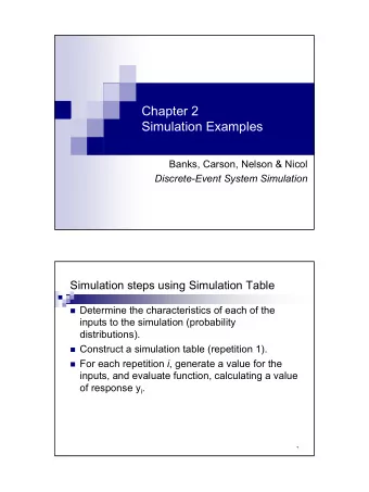
Outline The simulations are carried out by following steps: Determine the input characteristics. Construct a simulation table. For each repetition i, generate a value for each input, evaluate the function, and calculate the value of the response y i. Simulation examples are in queueing, inventory, reliability and network analysis. 3
Simulation of Queueing Systems A queueing system is described by its calling population, nature of arrivals, service mechanism, system capacity and the queueing discipline (details in Chapter 6.) A simple single-channel queuing system: In a single-channel queue: The calling population is infinite. Arrivals for service occur one at a time in a random fashion, once they join the waiting line, they are eventually served. Arrivals and services are defined by the distribution of the time between arrivals and service times. Key concepts: The system state is the number of units in the system and the status of the server (busy or idle). An event is a set of circumstances that causes an instantaneous change in the system state, e.g., arrival and departure events. The simulation clock is used to track simulated time. 4
Simulation of Queueing Systems If a unit has just completed service, the simulation proceeds in the manner shown below: The flow diagram for the arrival event: 5
Simulation of Queueing Systems Potential unit actions upon arrival: Server out comes after the completion of service: 6
Simulation of Queueing Systems Event list: to help determine what happens next. Tracks the future times at which different types of events occur. (this chapter simplifies the simulation by tracking each unit explicitly.) Events usually occur at random times. The randomness needed to imitate real life is made possible through the use of random numbers, they can be generated using: Random digits tables: form random numbers by selecting the proper number of digits and placing a decimal point to the left of the value selected. Simulation packages and spreadsheets. Details in chapter 7. 7
Simulation of Queueing Systems Single-channel queue illustration Assume that the times between arrivals were generated by rolling a die 5 times and recording the up face. Input generated: The 1 st customer is assumed to arrive at clock time 0. 2 nd customer arrives two time units later (at clock time 2), and so on. Assume the only possible service times are 1,2,3 and 4 time units and they are equally likely to occur. Input generated: 8
Simulation of Queueing Systems Resulting simulation table emphasizing clock times: Another presentation method, by chronological ordering of events: 9
Simulation of Queueing Systems Grocery store example: with only one checkout counter. Customers arrive at random times from 1 to 8 minutes apart, with equal probability of occurrence: The service times vary from 1 to 6 minutes, with probabilities: 10
Grocery Store Example [Simulation of Queueing Systems] To analyze the system by simulating arrival and service of 100 customers. Chosen for illustration purpose, in actuality, 100 customers is too small a sample size to draw any reliable conclusions. Initial conditions are overlooked to keep calculations simple. A set of uniformly distributed random numbers is needed to generate the arrivals at the checkout counter: Should be uniformly distributed between 0 and 1 . Successive random numbers are independent. With tabular simulations, random digits can be converted to random numbers. List 99 random numbers to generate the times between arrivals. Good practice to start at a random position in the random digit table and proceed in a systematic direction (never re-use the same stream of digits in a given problem) 11
Grocery Store Example [Simulation of Queueing Systems] 12
Grocery Store Example [Simulation of Queueing Systems] 13
Grocery Store Example [Simulation of Queueing Systems] Generated time-between-arrivals: Using the same methodology, service times are generated: 14
Grocery Store Example [Simulation of Queueing Systems] For manual simulation, Simulation tables are designed for the problem at hand, with columns added to answer questions posed: 15
Grocery Store Example [Simulation of Queueing Systems] Tentative inferences: About half of the customers have to wait, however, the average waiting time is not excessive. The server does not have an undue amount of idle time. Longer simulation would increase the accuracy of findings. Note: The entire table can be generated using the Excel spreadsheet for Example 2.1 at www.bcnn.net. 16
Grocery Store Example [Simulation of Queueing Systems] 17
Grocery Store Example [Simulation of Queueing Systems] Expected service time: 18
Able-Baker Call Center Example [ Simulation of Queueing Systems] A computer technical support center with two personnel taking calls and provide service. Two support staff: Able and Baker (multiple support channel). A simplifying rule: Able gets the call if both staff are idle. Goal: to find how well the current arrangement works. Random variable: Arrival time between calls Service times (different distributions for Able and Baker). A simulation of the first 100 callers are made More callers would yield more reliable results, 100 is chosen for purposes of illustration. 19
Able-Baker Call Center Example [ Simulation of Queueing Systems] 20
Able-Baker Call Center Example [ Simulation of Queueing Systems] 21
Able-Baker Call Center Example [ Simulation of Queueing Systems] The steps of simulation are implemented in a spreadsheet available on the website (www.bcnn.net). In the first spreadsheet, we found the result from the trial: 62% of the callers had no delay 12% had a delay of one or two minutes. 22
Able-Baker Call Center Example [ Simulation of Queueing Systems] In the second spreadsheet, we run an experiment with 400 trials (each consisting of the simulation of 100 callers) and found the following: 19% of the average delays are longer than two minutes. Only 2.75% are longer than 3 minutes. 23
Simulation of Inventory Systems A simple inventory system, an (M, N) inventory system: Periodic review of length, N , at which time the inventory level is checked. An order is made to bring the inventory up to the level M . At the end of the i th review period, an order quantity, Q i , is placed. 24
Simulation of Inventory Systems A simple inventory system (cont.): Total cost (or profit) of an inventory system is the performance measure . Carrying stock in inventory has associated cost. Purchase/replenishment has order cost. Not fulfilling order has shortage cost. 25
Simulation of Inventory Systems The News Dealer’s Example: A classical inventory problem concerns the purchase and sale of newspapers. News stand buys papers for 33 cents each and sells them for 50 cents each. Newspaper not sold at the end of the day are sold as scrap for 5 cents each. Newspaper can be purchased in bundles of 10 (can only buy 10, 20, … 50, 60 … ) Random Variables: Types of newsdays. Demand. 26
News Dealer’s Example [Simulation of Inventory Systems] Three types of newsdays: “good” ; “fair” ; “poor” ; with probabilities of 0.35, 0.45 and 0.20, respectively. 27
News Dealer’s Example [Simulation of Inventory Systems] Simulate the demands for papers over 20-day time period to determine the total profit under a certain policy, e.g. purchase 70 newspaper The policy is changed to other values and the simulation is repeated until the best value is found. 28
News Dealer’s Example [Simulation of Inventory Systems] 29
News Dealer’s Example [Simulation of Inventory Systems] From Excel: running the simulation for 400 trials (each for 20 days) Average total profit = $137.61. Only 45 of the 400 results in a total profit of more than $160. 30
News Dealer’s Example [Simulation of Inventory Systems] First two histograms of daily profit The manual solution had a profit of $131.00, not far from the average over 400 days, $137.61. 31
Other Examples of Simulation A Reliability Problem: A machine with different failure types of which repairman is called to install or repair the part. Downtime for the mill : $10 per minute. On-site cost of the repairperson : $30 per hour. It takes 20 minutes to change one bearing , 30 minutes to change two bearings , and 40 minutes to change three bearings. The delay time of the repairperson’s arriving : Delay Probability Cumulative Random digit Time(Minutes) Probability assignment 5 0.6 0.6 1 - 6 10 0.3 0.9 7 - 9 15 0.1 1 0 32
Recommend
More recommend
Explore More Topics
Stay informed with curated content and fresh updates.
