Simulating Biomolecules with Variable Protonation State: Constant-pH - PowerPoint PPT Presentation
Simulating Biomolecules with Variable Protonation State: Constant-pH Molecular Dynamics Simulations with NAMD Brian Radak University of Illinois at UrbanaChampaign Beckman Institute and Center for Macromolecular Modeling & Bioinformatics
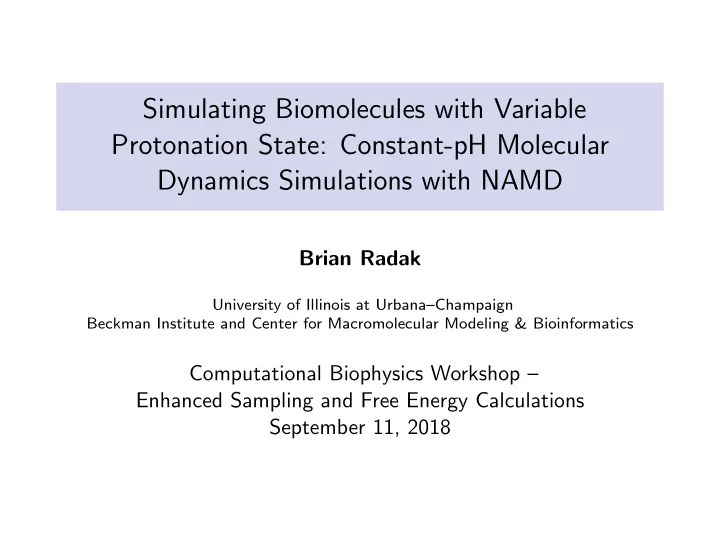
Simulating Biomolecules with Variable Protonation State: Constant-pH Molecular Dynamics Simulations with NAMD Brian Radak University of Illinois at Urbana–Champaign Beckman Institute and Center for Macromolecular Modeling & Bioinformatics Computational Biophysics Workshop – Enhanced Sampling and Free Energy Calculations September 11, 2018
Acknowledgements (other people to blame) Univ of Chicago ◮ Benoˆ ıt Roux ◮ Donghyuk Suh ALCF ◮ Wei Jiang Theta Early Science Program UIUC ◮ Dave Hardy ◮ Jim Phillips ◮ Chris Chipot ◮ Abhi Singharoy (ASU) ◮ Shashank Pant ◮ Emad Tajkhorshid
pH Effects in Biochemistry Casey, et al Nat Rev Mol Cell Biol , 2010 enzyme rate vs. pH 6.0 golgi endosome 6.7 5.5-6.5 general general mitochondria acid base fractional population lysosome k opt 8.0 rate constant 4.7 endoplasmic nucleus reticulum cytosol 7.2 pK a,acid pK a,opt pK a,base pH variability of pH by region cancerous normal + pHe 7.5 6.9 pH gradients at cell surfaces + pHi 7.2 7.5 Webb, et al Nat Rev Cancer , 2011
Constant pH and the semi-grand canonical ensemble ◮ Conventional MD samples a canonical ensemble: � d x e − β U ( x ) Q = ◮ Constant-pH MD samples a semi-grand canonical ensemble: � Q λ 10 − n λ pH Ξ(pH) = λ ∈S The added interaction is between the number of protons, n λ , and a pH bath. λ is a new variable designating the protonation state.
Networks of protonation states − H + − H + E-R − E-R − E-R 1 H:R 2 H 1 :R 2 H E-R 1 H:R 2 H 1 :R 2 H − H + − H + − H + − H + − H + − H + E-R 1 H:R − E-R − 1 :R − E-R 1 H:R − E-R − 1 :R − 2 2 2 2 constant pH MD conventional MD
Networks of protonation states − H + − H + E-R − E-R − E-R 1 H:R 2 H 1 :R 2 H E-R 1 H:R 2 H 1 :R 2 H − H + − H + − H + − H + − H + − H + E-R 1 H:R − E-R − 1 :R − E-R 1 H:R − E-R − 1 :R − 2 2 2 2 constant pH MD conventional MD 2 N N = 1 2 3 4
pH as a thermodynamic force ◮ Classical MD utilizes mechanical forces F = −∇ U [ x ( t )] ◮ pH may be regarded as a thermodynamic force 1 ∂ ln Ξ pH = − ln 10 ∂ n λ Mechanical forces – deterministic/stochastic dynamics Thermodynamic forces – probabilistic “dynamics” P λ (pH) ∝ Q λ 10 − n λ pH
How do we define nodes in the network? Consider a system with m sites:
Protonation state probabilities/populations � d x A ( x , λ ) e − β U ( x ; λ ) 10 − n λ pH � λ ∈S � A ( x , λ ) � pH = Ξ(pH) P λ s = � λ s � pH – the probability that site s is occupied There are two kinds of terms in the summation, λ s = 0 / 1 Ξ(pH) = Ξ 0 (pH) + Ξ 1 (pH)10 − pH thus, Ξ 1 (pH)10 − pH 1 � λ s � pH = Ξ 0 (pH) + Ξ 1 (pH)10 − pH = 1 + Ξ 0 (pH) Ξ 1 ( pH ) 10 pH
Connection to thermodynamics 1 � λ s � pH = 1 + Ξ 0 (pH) Ξ 1 ( pH ) 10 pH compares to the Henderson-Hasselbalch equation such that p K a (pH) = − log Ξ 0 (pH) Ξ 1 (pH) , except that now p K a (pH) is pH dependent . One often uses the approximation: � � p K a ( pH ) ≈ p K (a) pH − p K (a) + (1 − n ) , a a where n is the Hill coefficient and p K (a) is the “apparent” p K a . a
Networks of protonation states − H + − H + E-R 1 H:R 2 H E-R − 1 :R 2 H E-R 1 H:R 2 H E-R − 1 :R 2 H − H + − H + − H + − H + − H + − H + E-R 1 H:R − E-R − 1 :R − E-R 1 H:R − E-R − 1 :R − 2 2 2 2 constant pH MD conventional MD We can now see that the fraction of simulation time spent in a given protonation state is directly impacted by the difference of the p K a of a residue/site and the pH.
That’s great – how do we sample the states? 1. Sample the configuration space of a given state ( i.e., sample x for a given Q λ ) 2. Change between protonation states according to the number of protons and the given pH ( i.e., sample λ and choose a new Q λ ) This may be regarded as a Gibbs sampling , whereby the configuration and state are sampled in an alternating fashion.
A problem! Environmental response ◮ (De)Protonation is a significant electrostatic event. ◮ Non-trivial reorganization of solvent, possibly solute. ◮ Naive sudden changes in protonation are likely to cause high energy configurations and/or steric clashes.
Possible solutions to the solvent clash problem auxillary implicit solvent continuous fractional proton discrete copy fractional proton
“Fast” alchemical growth ◮ Swap the protonation state by using time-dependent interactions. ◮ Gradually stronger interactions will induce solvent response. ◮ Clashes are avoided by using the natural dynamics of the model.
The neMD/MC constant pH paradigm ◮ Drive alchemical growth with nonequilibrium work ◮ Accept/reject with a generalized Metropolis criterion Stern J Chem Phys , 2007 ; Chen & Roux J Chem Theory Comput , 2015 ; Radak, et al. J Chem Theory Comput , 2017
The neMD/MC constant pH paradigm ! =2/3 neMD alchemical growth removal of auxiliary MC sample of auxiliary coordinates coordinates ! =0 ! =1 ! =1/3 ◮ Drive alchemical growth with nonequilibrium work ◮ Accept/reject with a generalized Metropolis criterion Stern J Chem Phys , 2007 ; Chen & Roux J Chem Theory Comput , 2015 ; Radak, et al. J Chem Theory Comput , 2017
Beyond Gibbs sampling: Hybrid MD and neMD/MC We now alternate conventional sampling with MD ( x ) and Metropolis Monte Carlo sampling ( x and λ ): ρ ( x , λ ) T ( x , λ → x ′ , λ ′ ) = ρ ( x ′ , λ ′ ) T ( x ′ , λ ′ → x , λ ) such that the neMD/MC transition probability is: 1 , ρ ( x ′ , λ ′ ) � � T ( x , λ → x ′ , λ ′ ) = min ρ ( x , λ ) � 1 , e − β W 10 − ∆ n pH � = min (If you’d like, MD uses the probability T ( x → x ′ ) = 1.)
Important considerations ◮ How long should I sample the equilibrium stage? ◮ How long should I sample the nonequilibrium stage? (the “switch time,” τ switch ) ◮ Rejecting a nonequilibrum trajectory is expensive, how can we avoid doing that so much?
The two-step “inherent” p K a algorithm T ( x , λ → x ′ , λ ′ ) = T ( i ) ( λ → λ ′ ) T ( s ) ( x → x ′ | λ → λ ′ ) 1 , 10 p K (i) � a ( λ , λ ′ ) − ∆ n pH � T ( i ) ( λ → λ ′ ) = min ◮ neMD/MC can be split into two parts 1. T ( i ) – only depends on λ and the pH – CHEAP 2. T ( s ) – depends on the switch ( W ) – COSTLY Chen & Roux J Chem Theory Comput , 2015 ; Radak, et al. J Chem Theory Comput , 2017
The two-step “inherent” p K a algorithm T ( x , λ → x ′ , λ ′ ) = T ( i ) ( λ → λ ′ ) T ( s ) ( x → x ′ | λ → λ ′ ) 1 , 10 p K (i) � a ( λ , λ ′ ) − ∆ n pH � T ( i ) ( λ → λ ′ ) = min ◮ neMD/MC can be split into two parts 1. T ( i ) – only depends on λ and the pH – CHEAP 2. T ( s ) – depends on the switch ( W ) – COSTLY ◮ Effort is shifted by estimating a parameter, p K (i) a ◮ Optimal efficiency achieved for exact p K a Chen & Roux J Chem Theory Comput , 2015 ; Radak, et al. J Chem Theory Comput , 2017
The two-step “inherent” p K a algorithm T ( x , λ → x ′ , λ ′ ) = T ( i ) ( λ → λ ′ ) T ( s ) ( x → x ′ | λ → λ ′ ) 1 , 10 p K (i) � a ( λ , λ ′ ) − ∆ n pH � T ( i ) ( λ → λ ′ ) = min ◮ neMD/MC can be split into two parts 1. T ( i ) – only depends on λ and the pH – CHEAP 2. T ( s ) – depends on the switch ( W ) – COSTLY ◮ Effort is shifted by estimating a parameter, p K (i) a ◮ Optimal efficiency achieved for exact p K a ◮ Dramatically improved performance on wide pH ranges! Chen & Roux J Chem Theory Comput , 2015 ; Radak, et al. J Chem Theory Comput , 2017
A graphical view of the inherent p K a algorithm 1.0 0.8 ...to be occupied probability ...to add 0.6 if unoccupied ...to remove 0.4 if occupied 0.2 0.0 pK a - 2 pK a - 1 pK a pK a + 1 pK a + 2 pH ◮ It’s silly to try to add/remove protons to/from acidic/basic residues at high/low pH ◮ Transitions are proposed in proportion to the estimated population.
What about after we’ve proposed a switch? ◮ A short switch will not change much and likely be rejected. ◮ A long switch is expensive (limit of a single switch – BAD). ◮ Since the switch success depends on the work, let’s analyze that.
Work and force fluctuations – a typical neMD/MC cycle τ mol τ switch 2 σ 0 2 force σ 0 force correlation work ∆ F 0 0 5 10 15 20 0 50 100 150 200 time (/ps) Radak & Roux J Chem Phys , 2016
Theoretical and Empirical Performance Analysis 1.0 20 near maximal mean acceptance probability acceptance probability 0.8 σ 2 0 τ mol transition rate (/ns -1 ) 15 τ opt ≤ 2 . 83475 0.6 10 ≤ 23 . 4% P opt 0.4 5 ≥ 0 . 66318 P opt 0.2 τ opt ≈ 11 ps k opt ≡ near minimal σ 2 τ opt 0 τ mol transition rate 0 0.0 0 10 20 30 40 50 60 1400 1600 1800 2000 switch time (/ps) ◮ High acceptance is good, but not naively optimizable ◮ The transition rate can be optimized within constraints Radak & Roux J Chem Phys , 2017 ; Radak, et al. J Chem Theory Comput , 2017
Recommend
More recommend
Explore More Topics
Stay informed with curated content and fresh updates.
