SIFT Features and Hough Transform Various slides from previous - PowerPoint PPT Presentation
CS4501: Introduction to Computer Vision SIFT Features and Hough Transform Various slides from previous courses by: D.A. Forsyth (Berkeley / UIUC), I. Kokkinos (Ecole Centrale / UCL). S. Lazebnik (UNC / UIUC), S. Seitz (MSR / Facebook), J. Hays
CS4501: Introduction to Computer Vision SIFT Features and Hough Transform Various slides from previous courses by: D.A. Forsyth (Berkeley / UIUC), I. Kokkinos (Ecole Centrale / UCL). S. Lazebnik (UNC / UIUC), S. Seitz (MSR / Facebook), J. Hays (Brown / Georgia Tech), A. Berg (Stony Brook / UNC), D. Samaras (Stony Brook) . J. M. Frahm (UNC), V. Ordonez (UVA).
Last Class – Interest Points • Corner Detection - Harris • Blob Detection – Laplacian of Gaussian / Difference of Gaussians (DoG)
Today’s Class • Blog Detection – Difference of Gaussians • SIFT Feature descriptor – Feature Matching • Hough Transform -> For Line Detection
Basic idea Convolve the image with a “blob filter” at multiple • scales and look for extrema of filter response in the resulting scale space T. Lindeberg. Feature detection with automatic scale selection. IJCV 30(2), pp 77-116, 1998. Slide by Svetlana Lazebnik
Blob filter • Laplacian of Gaussian: Circularly symmetric operator for blob detection in 2D ¶ ¶ 2 2 g g Ñ = + 2 g ¶ ¶ 2 2 x y
Blob detection minima = * maxima • Find maxima and minima of blob filter response in space and scale Source: N. Snavely
Blob at multiple scales – Option 1 = * = * = *
Apply Non-Max Suppression – Show blobs as circles
Scale-space blob detector: Example Slide by Svetlana Lazebnik
Scale-space blob detector: Example Slide by Svetlana Lazebnik
Blog at Multiple Scales: Option 2 Slide by Svetlana Lazebnik
Scale-space blob detector 1. Convolve image with scale-normalized Laplacian at several scales 2. Find maxima of squared Laplacian response in scale-space Slide by Svetlana Lazebnik
Scale-space blob detector: Example Slide by Svetlana Lazebnik
Efficient implementation Approximating the Laplacian with a difference of Gaussians: • ( ) = s 2 s + s L G ( , , ) x y G ( , , ) x y xx yy (Laplacian) = s - s DoG G x y k ( , , ) G x y ( , , ) (Difference of Gaussians) Slide by Svetlana Lazebnik
Efficient implementation David G. Lowe. "Distinctive image features from scale-invariant keypoints.” IJCV 60 (2), pp. 91-110, 2004.
Gaussian Pyramid – DoG pyramid David G. Lowe. "Distinctive image features from scale-invariant keypoints.” IJCV 60 (2), pp. 91-110, 2004. Figure from Workload analysis and efficient OpenCL-based implementation of SIFT algorithm on a smartphone •Guohui Wang, Blaine Rister, Joseph R. Cavallaro
Gaussian Pyramid David G. Lowe. "Distinctive image features from scale-invariant keypoints.” IJCV 60 (2), pp. 91-110, 2004. Figure from Workload analysis and efficient OpenCL-based implementation of SIFT algorithm on a smartphone •Guohui Wang, Blaine Rister, Joseph R. Cavallaro
Same results Slide by Svetlana Lazebnik
Locations + Scales + Orientations D. Lowe, Distinctive image features from scale-invariant keypoints, IJCV 60 (2), pp. 91-110, 2004.
Eliminating rotation ambiguity • To assign a unique orientation to circular image windows: Create histogram of local gradient directions in the • patch • Assign canonical orientation at peak of smoothed histogram 2 p 0 Slide by Svetlana Lazebnik
From keypoint detection to keypoint representation (feature descriptors) Figure by Svetlana Lazebnik
SIFT descriptors • Inspiration: complex neurons in the primary visual cortex D. Lowe. Distinctive image features from scale-invariant keypoints. IJCV 60 (2), pp. 91-110, 2004.
From keypoint detection to keypoint representation (feature descriptors) Compare SIFT feature vectors instead Figure by Svetlana Lazebnik
SIFT Feature Matching Rice Hall at UVA
JiaWang Bian, Wen-Yan Lin, Yasuyuki Matsushita, Sai-Kit Yeung, Tan Dat Nguyen, Ming-Ming Cheng GMS: Grid-based Motion Statistics for Fast, Ultra-robust Feature Correspondence IEEE CVPR, 2017 The method has been integrated into OpenCV library (see xfeatures2d in opencv_contrib).
A hard keypoint matching problem NASA Mars Rover images
Answer below (look for tiny colored squares…) NASA Mars Rover images with SIFT feature matches Figure by Noah Snavely
Feature Descriptors Zoo • SIFT (under a patent) Proposed around 1999 • SURF (under a patent too – I think) • BRIEF • ORB (seems free as it is OpenCV’s preferred) • BRISK • FREAK • FAST • KAZE • LIFT (Most recently proposed at ECCV 2016)
How to do Line Detection?
How to do Line Detection? x = 12px x = 38px x = 68px y = 16px y = 20px y = 56px
Idea: Sobel First! x = 12px x = 38px x = 68px y = 16px y = 20px y = 56px
Idea: Sobel First! x = 12px x = 38px x = 68px y = 16px y = 20px y = 56px
Idea: Then Count Pixels that support each line hypothesis. x = 12px x = 38px x = 68px y = 16px y = 20px y = 56px
Idea: Then Count Pixels that support each line hypothesis. x = 12px x = 38px x = 68px y = 16px y = 20px count (sum) y = 56px count (sum)
Problem with this? x = 12px x = 38px x = 68px y = 16px y = 20px count (sum) y = 56px count (sum)
What if you’re given this instead?
How do we get this?
Furthermore. How do we get this!? y= -2x + 30 y= x + 10 y= -2x + 20 y= x + 7 y= -2x + 10 y= x - 5
Hough transform • An early type of voting scheme for Detecting Lines • General outline: • Discretize parameter space into bins • For each feature point in the image, put a vote in every bin in the parameter space that could have generated this point • Find bins that have the most votes Image space Hough parameter space P.V.C. Hough, Machine Analysis of Bubble Chamber Pictures, Proc. Int. Conf. High Energy Accelerators and Instrumentation, 1959 Slides by Svetlana Lazebnik
Hough Transform: Let’s again apply Sobel first
Hough Transform: Let’s again apply Sobel first
Then let’s count but now in a 2D array ! = #$ + & # & Count all points intersecting with all lines with m = (0, inf), b = [-B-min, B-max]
Parameter space representation •Problems with the (m,b) space: • Unbounded parameter domains • Vertical lines require infinite m
Parameter space representation • Problems with the (m,b) space: • Unbounded parameter domains • Vertical lines require infinite m • Alternative: polar representation q + q = r x cos y sin
Then let’s count but now in a 2D array ! cos % + ' sin % = + + % Count all points intersecting with all lines with rho = (-diagonal, diagonal), theta = [0, 180]
Hough Transform Algorithm outline • Initialize accumulator H to all zeros • For each feature point (x,y) ρ in the image For θ = 0 to 180 ρ = x cos θ + y sin θ H(θ, ρ) = H(θ, ρ) + 1 θ end end • Find the value(s) of (θ, ρ) where H(θ, ρ) is a local maximum • The detected line in the image is given by ρ = x cos θ + y sin θ Slide by Svetlana Lazebnik
• Each point (x,y) in Image Space will add a sinusoid in the Hough Transform ( q , r ) parameter space
Basic illustration votes features
Hough Transform for an Actual Image
Edges using threshold on Sobel’s magnitude
Hough Transform (High Resolution) ' = − ℎ ) + + ) ' = 0 ℎ ) + + ) ' = ! = −90 & ! = 90 & ! = 0
Hough Transform (After threshold) ' = − ℎ ) + + ) ' = 0 ℎ ) + + ) ' = ! = −90 & ! = 90 & ! = 0
Hough Transform (After threshold) ' = − ℎ ) + + ) Vertical lines ' = 0 ℎ ) + + ) ' = ! = −90 & ! = 90 & ! = 0
Hough Transform (After threshold) ' = − ℎ ) + + ) Vertical lines ' = 0 ℎ ) + + ) ' = ! = −90 & ! = 90 & ! = 0
Hough Transform with Non-max Suppression ' = − ℎ ) + + ) ' = 0 ℎ ) + + ) ' = ! = −90 & ! = 90 & ! = 0
Back to Image Space – with lines detected ! = − $%&' , q + q = r &()' * + cos sin x y &()'
Hough transform demo
Incorporating image gradients • Recall: when we detect an edge point, we also know its gradient direction • But this means that the line is uniquely determined! • Modified Hough transform: For each edge point (x,y) • θ = gradient orientation at (x,y) ρ = x cos θ + y sin θ H(θ, ρ) = H(θ, ρ) + 1 end Slide by Svetlana Lazebnik
Hough transform for circles image space Hough parameter space r y + Ñ ( x , y ) r I ( x , y ) (x,y) x - Ñ ( x , y ) r I ( x , y ) x y Slide by Svetlana Lazebnik
Hough transform for circles •Conceptually equivalent procedure: for each (x,y,r), draw the corresponding circle in the image and compute its “support” r x y Is this more or less efficient than voting with features? Slide by Svetlana Lazebnik
Questions? 62
Recommend
More recommend
Explore More Topics
Stay informed with curated content and fresh updates.
