Feature Detection and Matching Shao-Yi Chien Department of - PowerPoint PPT Presentation
Feature Detection and Matching Shao-Yi Chien Department of Electrical Engineering National Taiwan University Fall 2019 1 References: Slides from Digital Visual Effects , Prof. Y.-Y. Chuang, CSIE, National Taiwan University
Speed Up Robust Feature (SURF) • Descriptor • Based on sum of Haar wavelet response • dx,dy : wavelet responses in x & y direction • 4x4 sub-region • Calculate Σ dx , Σ dy, Σ |dx|, Σ |dy| • 4*4*4 = 64 dimensions • 4*4*5*5=400 times calculation for an interest point • Irregular pattern Σ dx dx dy Σ |dx| Σ dy Σ |dy| 47
Feature Matching How to define the difference between two features f 1 , f 2 ? • Simple approach is SSD(f 1 , f 2 ) • sum of square differences between entries of the two descriptors • can give good scores to very ambiguous (bad) matches f 1 f 2 I 1 I 2 48
Feature Matching How to define the difference between two features f 1 , f 2 ? • Better approach: ratio distance = SSD(f 1 , f 2 ) / SSD(f 1 , f 2 ’) • f 2 is best SSD match to f 1 in I 2 f 2 ’ is 2 nd best SSD match to f 1 in I 2 • • gives small values for ambiguous matches ' f 1 f 2 f 2 I 1 I 2 49
Feature Matching • Matching? The difference < threshold • How to evaluate? • TP: true positives • FN: false negatives • FP: false positives • TN: true negatives 50
Feature Matching • How to evaluate? 𝑈𝑄 + 𝐺𝑂 = 𝑈𝑄 𝑈𝑄 𝑈𝑄𝑆 = • True positive rate (TPR), recall 𝑄 𝐺𝑄 + 𝑈𝑂 = 𝐺𝑄 𝐺𝑄 • False positive rate (FPR), false alarm 𝐺𝑄𝑆 = 𝑂 • Positive predictive value (PPV), precision 𝑈𝑄 + 𝐺𝑄 = 𝑈𝑄 𝑈𝑄 𝑄𝑄𝑊 = 𝑄′ • Accuracy (ACC) 𝐵𝐷𝐷 = 𝑈𝑄 + 𝑈𝑂 𝑄 + 𝑂 51
𝑈𝑄 Feature Matching 𝑈𝑄𝑆 = 𝑈𝑄 + 𝐺𝑂 True positive rate (TPR) 𝐺𝑄 𝐺𝑄𝑆 = • How to evaluate? 𝐺𝑄 + 𝑈𝑂 False positive rate (FPR) 𝑈𝑄 Positive predictive value (PPV) 𝑄𝑄𝑊 = 𝑈𝑄 + 𝐺𝑄 Accuracy (ACC) 𝐵𝐷𝐷 = 𝑈𝑄 + 𝑈𝑂 ROC curve (Receiver Operating Characteristic) 𝑄 + 𝑂 52
Feature Matching • Efficient matching • Full search • Indexing structure • Multi-dimensional hashing • Locality sensitive hashing (LSH) • K-d tree 53
Applications Features are used for: • Image alignment (e.g., mosaics) • 3D reconstruction • Motion tracking • Object recognition • Indexing and database retrieval • Robot navigation • … other 54
Object Recognition (David Lowe) 55
BRIEF (ECCV 2010) • We define test 𝜐 on patch 𝐪 of size 𝑇 × 𝑇 as • where 𝐪(𝐲) is the pixel intensity in a smoothed version of 𝐪 at 𝐲 = (𝑣, 𝑤)⊤ . • Choosing a set of 𝑜 𝑒 (𝑦, 𝑧) -location pairs uniquely defines a set of binary tests. • We take our BRIEF descriptor to be the 𝑜 𝑒 -dimensional bitstring 56
57
BRISK (ICCV2011)
FREAK (CVPR 2012) • Retinal sampling pattern • Coarse-to-fine descriptor • How to select pairs? • Learn the best pairs from training data
FREAK (CVPR 2012)
ORB: An efficient alternative to SIFT or SURF • ORB = oFAST + rBRIEF • oFAST: FAST Keypoint Orientation • rBRIEF: Rotation-Aware Brief E. Rublee, V. Rabaud, K. Konolige and G. Bradski , “ORB: An efficient alternative to SIFT or SURF,” in Proc. 2011 International Conference on Computer Vision , Barcelona, 2011. 61
1 Rosten, Edward, and Tom Drummond. "Machine learning for high-speed corner detection." Computer Vision – ECCV 2006. FAST 1 • Features from Accelerated Segment Test. • The segment test criterion operates by considering a circle of sixteen pixels around the corner candidate p. • The original detector classifies p as a corner if there exists a set of n contiguous pixels in the circle which are all brighter than the intensity of the candidate pixel I p + t, or all darker than I p - t. 62
Orientation by Intensity Centroid • Moments of a patch • with these moments we may find the centroid • We can construct a vector from the corner's center, 𝑃 , to the centroid, 𝑃𝐷 . 63
Rotation Measure • IC: intensity centroid • MAX chooses the largest gradient in the keypoint patch • BIN forms a histogram of gradient directions at 10 degree intervals, and picks the maximum bin. 64
Steered BRIEF • Steer BRIEF according to the orientation of keypoints. • Using the patch orientation 𝜄 and the corresponding rotation matrix R 𝜄 , we construct a "steered" version S 𝜄 of S : • Now the steered BRIEF operator becomes 65
Learning Good Binary Features • The algorithm is: 66
Results (1/3) • Matching performance of SIFT, SURF, BRIEF with FAST, and ORB (oFAST +rBRIEF) under synthetic rotations with Gaussian noise of 10. Po-Chen Wu ( 吳柏辰 ) 67 Media IC & System Lab
Results (2/3) • Matching behavior under noise for SIFT and rBRIEF. The noise levels are 0, 5, 10, 15, 20, and 25. SIFT performance degrades rapidly, while rBRIEF is relatively unaffected. Po-Chen Wu ( 吳柏辰 ) 68 Media IC & System Lab
Results (3/3) • Test on real-world images: Po-Chen Wu ( 吳柏辰 ) 69 Media IC & System Lab
Computation Time • The ORB system breaks down into the following times per typical frame of size 640x480. Intel i7 2.8 GHz Pascal 2009 dataset 2686 images at 5 scales Po-Chen Wu ( 吳柏辰 ) 70 Media IC & System Lab
OpenCV 2.4.9 • Detector • "FAST" – FastFeatureDetector • "STAR" – StarFeatureDetector • "SIFT" – SIFT (nonfree module) • "SURF" – SURF (nonfree module) • "ORB" – ORB • "BRISK" – BRISK • "MSER" – MSER • "GFTT" – GoodFeaturesToTrackDetector • "HARRIS" – GoodFeaturesToTrackDetector with Harris detector enabled • "Dense" – DenseFeatureDetector • "SimpleBlob" – SimpleBlobDetector Po-Chen Wu ( 吳柏辰 ) 71 Media IC & System Lab
OpenCV 2.4.9 • Descriptor • "SIFT" – SIFT • "SURF" – SURF • "BRIEF" – BriefDescriptorExtractor • "BRISK" – BRISK • "ORB" – ORB • "FREAK" – FREAK Po-Chen Wu ( 吳柏辰 ) 72 Media IC & System Lab
Edges and Lines 73
Y. Cao, C. Wang, L. Zhang and L. Zhang, "Edgel index for large-scale sketch- based image search," in Proc. CVPR 2011. 74
Edge Detection • Canny edge detector • The most widely used edge detector • The best you can find in existing tools like MATLAB, OpenCV … • Algorithm: • Apply Gaussian filter to reduce noise • Find the intensity gradients of the image • Apply non-maximum suppression to get rid of false edges • Apply double threshold to determine potential edges • Track edge by hysteresis : suppressing weak edges that are not connected to strong edges 75
Hysteresis • Find connected components from strong edge pixels to finalize edge detection 76
Hough Transform 77
Hough Transform • Vote in 𝜄, 𝑠 space • (Many choices) 78
Hough Transform • Clear the accumulator array • For each detected edgel at location (𝑦, 𝑧) and orientation 𝜄 = 𝑢𝑏𝑜 −1 𝑜 𝑧 /𝑜 𝑦 , compute the value of 𝑒 = 𝑦𝑜 𝑦 + 𝑧𝑜 𝑧 and increment the accumulator corresponding to (𝜄, 𝑒) • Find the peaks in the accumulator corresponding to lines • Optionally re-fit the lines to the constituent edgels 79
Deep Features 80
Deep Features • Features extracted from Deep Neural Network • Ex. Deep Face (CVPR2014)
Deep Features Loss function: E. Simo-Serra, E. Trulls, L. Ferraz, I. Kokkinos, P. Fua, and F. Moreno-Noguer, “Discriminative learning of deep convolutional feature point descriptors,” in Proc. 82 ICCV 2015 .
Deep Features E. Simo-Serra, E. Trulls, L. Ferraz, I. Kokkinos, P. Fua, and F. Moreno-Noguer, “Discriminative learning of deep convolutional feature point descriptors,” in Proc. ICCV 2015 . 83
Appendix: MPEG-7 Descriptors 84
Introduction • MPEG-7 is a standard for describing features of multimedia content • MPEG- 7 provides the world’s richest set of audio - visual descriptions • Comprehensive scope of data interoperability • Based on XML 85
Introduction • General visual descriptors • Color • Texture • Shape • Motion • Domain-specific visual descriptors • Face recognition descriptors 86
What is Standardized? • Only define the descriptions • Not standardize how to produce the descriptions • Not standardize how to use the descriptions • Only define what is needed for the interoperability of MPEG-7 enabled systems 87
What is Standardized? 88
Color Descriptors • Color Space Descriptor • Dominant Color Descriptor • Scalable Color Descriptor • Group of Frames (or Pictures) Descriptor • Color Structure Descriptor • Color Layout Descriptor 89
Example: Dominant Color Descriptor (1) • Compact description • Browsing of image databases based on single or several color values • Definition: • F = {( c i , p i , v i ), s}, (i = 1, 2, …, N) (N < 9) • c i : color value vector (default color space: RGB) • p i : percentage ( ) = p 1 i i • v i : optional color variance • s : spatial coherency 90
Dominant Color Descriptor (2) • Binary syntax of DCD Field Number of Bits Meaning NumberofColors 3 Specifies number of dominant colors SpatialCoherency 5 Spatial Coherency Value Percentage[] 5 Normalized percentage associated with each dominant color ColorVariance[][] 1 Color variance of each dominant color Index[][] 1 — 12 Dominant color values 91
Dominant Color Descriptor (3) • Extraction: • Clustering is performed in a perceptually uniform color space (Lloyd algorithm) • Distortion : = − 2 D h ( n ) x ( n ) c , x ( n ) C • x (n) : the color vector at pixel n i i i n • h(n) : perceptual weight for pixel n • c i : centroid of cluster C i = h ( n ) x ( n ) c , x ( n ) C i i h ( n ) 92
Dominant Color Descriptor (4) • Extraction: • The procedure is initialized with one cluster consisting of all pixels and one representative color computed as the centroid of the cluster • The algorithm then follows a sequence of centroid calculation and clustering steps until a stopping criterion (minimum distortion or maximum number of iterations) 93
Dominant Color Descriptor (5) • Extraction: • Spatial coherency (s): • 4 connectivity connected component analysis • Individual spatial coherence: normalized average number of the connected pixels of each dominant color • s = (individual spatial coherence) i p • S is nonuniformly quantized to 5 bits, i i 31 means highest confidence 1 means no confidence 0 means not computed 94
Dominant Color Descriptor (6) • Similarity Matching: • Number of representative colors is small, one can first search the database for each of the representative color separately, then combine. 95
Dominant Color Descriptor (7) • Similarity Matching: • Consider 2 DCDs : • • Dissimilarity (D): = − d k,l : d c c is the Euclidean distance between tw o colors k , l k l = d T max d 96
Dominant Color Descriptor (8) • Similarity Matching: • Dissimilarity (D s ): w 1 = 0.3, w 2 = 0.7 (recommanded) • Dissimilarity (D v ): 97
Dominant Color Descriptor (9) • Similarity Matching Results: 98
Texture Descriptors • Homogeneous Texture Descriptor (HTD) • Texture Browsing Descriptor (TBD) • Edge Histogram Descriptor (EHD) 99
Homogeneous Texture Descriptor = HTD [ f , f , e , e ,..., e , d , d ,... d ] DC SD 1 2 30 1 2 30 62 numbers (496 bits) Texture feature channels modeled using the Gabor functions in the polar frequency domain Channels used in computing the HTD
Recommend
More recommend
Explore More Topics
Stay informed with curated content and fresh updates.
