Matching and Image Alignment Computer Vision Fall 2018 Columbia - PowerPoint PPT Presentation
Matching and Image Alignment Computer Vision Fall 2018 Columbia University Feature Matching 1. Find a set of distinctive key- points 2. Define a region around each keypoint 3. Extract and normalize the region content 4. Compute a
Matching and Image Alignment Computer Vision Fall 2018 Columbia University
Feature Matching 1. Find a set of distinctive key- points 2. Define a region around each keypoint 3. Extract and normalize the region content 4. Compute a local descriptor from the normalized region 5. Match local descriptors Slide credit: James Hays
SIFT Review
Corner Detector: Basic Idea “flat” region: “edge”: “corner”: no change in any no change along the significant change in direction edge direction all directions Defn: points are “matchable” if small shifts always produce a large SSD error Source: Deva Ramanan
Scaling Corner All points will be classified as edges
What Is A Useful Signature Function f ? • “ Blob ” detector is common for corners – - Laplacian (2 nd derivative) of Gaussian (LoG) Scale space Function response Image blob size K. Grauman, B. Leibe
Coordinate frames Represent each patch in a canonical scale and orientation (or general affine coordinate frame) Source: Deva Ramanan
Find dominant orientation Compute gradients for all pixels in patch. Histogram (bin) gradients by orientation 0 2 π Source: Deva Ramanan
Computing the SIFT Descriptor Histograms of gradient directions over spatial regions \ Source: Deva Ramanan
Post-processing 1. Rescale 128-dim vector to have unit norm x x ∈ R 128 x = || x || , “invariant to linear scalings of intensity” 2. Clip high values x := min( x, . 2) x x := || x || approximate binarization allows for for flat patches with small gradients to remain stable Source: Deva Ramanan
Matching
Panoramas Slide credit: Olga Russakovsky
Gigapixel Images danielhartz.com
Look into the Past Slide credit: Olga Russakovsky
Can you find the matches? NASA Mars Rover images Slide credit: S. Lazebnik
NASA Mars Rover images with SIFT feature matches Figure by Noah Snavely Slide credit: S. Lazebnik
Discussion • Design a feature point matching scheme. • Two images, I 1 and I 2 • Two sets X 1 and X 2 of feature points � ( 1 ) ( 1 ) – Each feature point x 1 has a descriptor x [ x , , x ] � 1 1 d • Distance, bijective/injective/surjective, noise, confidence, computational complexity, generality … Slide credit: James Hays
Distance Metric • Euclidean distance: • Cosine similarity: Wikipedia
Matching Ambiguity ? Locally, feature matches are ambiguous => need to fit a model to find globally consistent matches Slide credit: James Hays
Feature Matching • Criteria 1: – Compute distance in feature space, e.g., Euclidean distance between 128-dim SIFT descriptors – Match point to lowest distance (nearest neighbor) • Problems: – Does everything have a match? Slide credit: James Hays
Feature Matching • Criteria 2: – Compute distance in feature space, e.g., Euclidean distance between 128-dim SIFT descriptors – Match point to lowest distance (nearest neighbor) – Ignore anything higher than threshold (no match!) • Problems: – Threshold is hard to pick – Non-distinctive features could have lots of close matches, only one of which is correct Slide credit: James Hays
Nearest Neighbor Distance Ratio Compare distance of closest (NN1) and second- closest (NN2) feature vector neighbor. 𝑂𝑂1 • If NN1 ≈ NN2, ratio 𝑂𝑂2 will be ≈ 1 -> matches too close. 𝑂𝑂1 • As NN1 << NN2, ratio 𝑂𝑂2 tends to 0. Sorting by this ratio puts matches in order of confidence. Threshold ratio – but how to choose? Slide credit: James Hays
Nearest Neighbor Distance Ratio • Lowe computed a probability distribution functions of ratios • 40,000 keypoints with hand-labeled ground truth Ratio threshold depends on your application ’ s view on the trade-off between the number of false positives and true positives! Lowe IJCV 2004
What is the transformation between these images?
Transformation Models • T ranslation only • Rigid body (translate+rotate) • Similarity (translate+rotate+scale) • AIne • Homography (projective)
Homogenous Coordinates Cartesian: Homogenous: ˜ P = ( x , y ) P = ( x , y ,1) Slide credit: Peter Corke
Homogenous Coordinates Cartesian: Homogenous: ˜ P = ( x , y ) P = ( x , y ,1) Homogenous: ˜ P = (˜ x , ˜ y , ˜ z ) Slide credit: Peter Corke
Homogenous Coordinates Cartesian: Homogenous: ˜ P = ( x , y ) P = ( x , y ,1) Cartesian: Homogenous: P = ( z ) x z , ˜ ˜ y ˜ P = (˜ x , ˜ y , ˜ z ) ˜ ˜ Slide credit: Peter Corke
Lines and Points are Duals p = ( ˜ z ) ˜ x , ˜ y , ˜ Point Equation of a Line: ℓ T ˜ ˜ p = 0 ℓ = ( l 1 , l 2 , l 3 ) ˜ l 1 ˜ x + l 2 ˜ y + l 3 ˜ z = 0 Slide credit: Peter Corke
p 1 = ( ˜ z 1 ) ˜ x 1 , ˜ y 1 , ˜ p 2 = ( ˜ z 2 ) ˜ x 2 , ˜ y 2 , ˜ ˜ ℓ Cross product of two points is a line: ˜ ℓ = ˜ p 1 × ˜ p 2 Slide credit: Peter Corke
˜ ℓ 2 p ˜ ˜ ℓ 1 Cross product of two lines is a point: p = ˜ ℓ 1 × ˜ ℓ 2 ˜ Slide credit: Peter Corke
Central Projection Model f Slide credit: Peter Corke
Central Projection Model f 0 0 x ˜ 0 0 1 ( Z ) X y ˜ p = = 0 f 0 Y z ˜ f Slide credit: Peter Corke
Central Projection Model f 0 0 x ˜ 0 0 1 ( Z ) X y ˜ p = = 0 f 0 Y z ˜ What if the camera moves? f Slide credit: Peter Corke
Review: 3D Transformations Slide credit: Deva Ramanan
Change of Coordinate System Slide credit: Deva Ramanan
Camera Projection X r 11 r 12 r 13 t x f 0 0 x ˜ Y r 21 r 22 r 23 t y y ˜ = f 0 0 Z z r 31 r 32 r 33 t x ˜ 0 0 1 1 Camera Camera World Intrinsics Extrinsics Coordinates
Camera Matrix Mapping points from the world to image coordinates is matrix multiplication in homogenous coordinates X C 11 C 12 C 13 C 14 x ˜ Y y ˜ C 21 C 22 C 23 C 24 = Z z ˜ C 31 C 32 C 33 C 34 1
Scale Invariance X C 11 C 12 C 13 C 14 x ˜ Y y ˜ C 21 C 22 C 23 C 24 = λ Z z ˜ C 31 C 32 C 33 C 34 1 x = ˜ x z = λ ˜ x y = ˜ y z = λ ˜ y ˜ λ ˜ z ˜ λ ˜ z
Normalized Camera Matrix X C 11 C 12 C 13 C 14 x ˜ Y y ˜ C 21 C 22 C 23 C 24 = Z z ˜ C 31 C 32 C 33 1 1
Homography Slide credit: Deva Ramanan
Projection of 3D Plane All points on the plane have Z = 0 X C 11 C 12 C 13 C 14 x ˜ Y y ˜ C 21 C 22 C 23 C 24 = 0 z ˜ C 31 C 32 C 33 1 1 Slide credit: Peter Corke
Projection of 3D Plane All points on the plane have Z = 0 X C 11 C 12 0 C 14 x ˜ Y y ˜ C 21 C 22 0 C 24 = 0 z ˜ C 31 C 32 0 1 1 Slide credit: Peter Corke
Planar Homography All points on the plane have Z = 0 1 ) = H ( H 11 H 12 H 14 x ˜ ( X X 1 ) y ˜ H 21 H 22 H 24 = Y Y z ˜ H 31 H 32 1 Slide credit: Peter Corke
Two-views of Plane = H 1 ( = H 2 ( x 1 ˜ x 2 ˜ X 1 ) X 1 ) y 1 y 2 ˜ ˜ Y Y z 1 ˜ z 2 ˜ If you know both H and (x1, y1), what is (x2, y2)? Slide credit: Deva Ramanan
Two-views of Plane = H 1 ( = H 2 ( x 1 ˜ x 2 ˜ X 1 ) X 1 ) y 1 y 2 ˜ ˜ Y Y z 1 ˜ z 2 ˜ x 2 x 1 ˜ ˜ = H 2 H − 1 y 2 ˜ y 1 ˜ 1 z 2 z 1 ˜ ˜ Slide credit: Deva Ramanan
Estimating Homography How many corresponding points do you need to estimate H? x 2 x 1 ˜ ˜ y 2 ˜ y 1 ˜ = H z 2 z 1 ˜ ˜ Slide credit: Deva Ramanan
Estimating Homography (details) Slide credit: Antonio Torralba
Estimating Homography (details) Slide credit: Antonio Torralba
Rectification Slide credit: Peter Corke
Rectification Slide credit: Peter Corke
Rectification Slide credit: Peter Corke
Rectification Slide credit: Peter Corke
Warping Slide credit: Peter Corke
Virtual Camera Slide credit: Peter Corke
Panoramas Slide credit: Olga Russakovsky
Special case of 2 views: rotations about camera center Can be modeled as planar transformations, regardless of scene geometry! Slide credit: Deva Ramanan
Derivation X 2 X 1 K 2 = R Y 2 Y 1 Relation between 3D camera coordinates: Z 2 Z 1 x 2 f 2 X 2 0 0 = y 2 f 2 Y 2 3D->2D projection: λ 2 0 0 Z 2 1 0 0 1 … x 2 x 1 = K 2 RK − 1 Combining both: λ y 2 y 1 1 1 1 Slide credit: Deva Ramanan
Take-home points for homographies x 2 a b c x 1 = y 2 d e f y 1 λ g h i 1 1 • If camera rotates about its center, then the images are related by a homography irrespective of scene depth. • If the scene is planar, then images from any two cameras are related by a homography. • Homography mapping is a 3x3 matrix with 8 degrees of freedom. Slide credit: Deva Ramanan
VLFeat’s 800 most confident matches among 10,000+ local features. Which matches should we use to estimate homography?
Least squares: Robustness to noise • Least squares fit to the red points: Slide credit: James Hays
Recommend
More recommend
Explore More Topics
Stay informed with curated content and fresh updates.
