Short-term GDP forecasting with a mixed frequency dynamic factor - - PowerPoint PPT Presentation

▶

Oct 08, 2022 443 likes •821 views

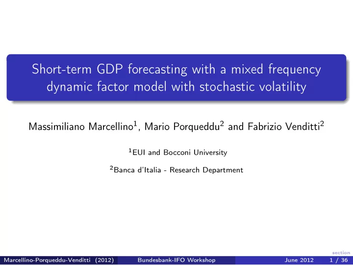
Short-term GDP forecasting with a mixed frequency dynamic factor model with stochastic volatility Massimiliano Marcellino 1 , Mario Porqueddu 2 and Fabrizio Venditti 2 1 EUI and Bocconi University 2 Banca dItalia - Research Department section

SLIDE 1

section

Short-term GDP forecasting with a mixed frequency dynamic factor model with stochastic volatility

Massimiliano Marcellino1, Mario Porqueddu2 and Fabrizio Venditti2

1EUI and Bocconi University 2Banca d’Italia - Research Department Marcellino-Porqueddu-Venditti (2012) Bundesbank-IFO Workshop June 2012 1 / 36

SLIDE 2

section

Plan of the talk

Motivation The model Estimation strategy An empirical application: forecasting euro area GDP Full sample results Daily business: some bayesian tools for nowcasting Out of sample: point and density forecast evaluation Some concluding remarks

Marcellino-Porqueddu-Venditti (2012) Bundesbank-IFO Workshop June 2012 2 / 36

SLIDE 3

section

Motivation 1

Interest in policy making and forecasting in probability distributions around a central forecast Fan charts: Bank of England, Bank of Canada, Norges Bank, SA Re- serve and Sveriges Riksbank, more recently Bank of Italy and also the US Fed (2008) Density forecasts are sensitive to shifts in the parameters of the model: Jore, Mitchell, and Vahey (2010), Clark (2011) Discrete breaks far away in the past: use sample split More recently: increasing interest in modeling small continuous breaks (time varying parameter models, Cogley and Sargent, 2003, Primiceri, 2005, large literature following) The Great Recession: spot light on volatility breaks (end to the Great Moderation?)

Marcellino-Porqueddu-Venditti (2012) Bundesbank-IFO Workshop June 2012 3 / 36

SLIDE 4

section

Motivation 2

Most of the work on density forecast/time varying models falls in the medium/long term forecasting literature Nowcasting/Short term forecasting is a world of its own

mixed frequency data ragged edge data different timeliness (soft/hard data)

There are existing tools that deal with the above issues but

No applications on density forecasts Time constant parameters (some allow for discrete random breaks in the mean: MS models)

Galvao (2009), STAR-MIDAS Guerin Marcellino (2011) MS-MIDAS Carriero, Clark, Marcellino (2012) U-MIDAS with stochastic volatility in the context of Nowcasting/Short term forecasting

Marcellino-Porqueddu-Venditti (2012) Bundesbank-IFO Workshop June 2012 4 / 36

SLIDE 5

section

Our contribution

Extend the mixed frequency factor model by Mariano and Murasawa (2003) to account for continuous shifts in volatility Derive some interesting tools:

Density forecasts / fan charts for GDP short term forecasts Probability distributions of the news content of indicator releases

Marcellino-Porqueddu-Venditti (2012) Bundesbank-IFO Workshop June 2012 5 / 36

SLIDE 6

section

Empirical application: forecasting euro area GDP

We document a dramatic increase in both common and idiosyncratic business cycle volatility in the euro area in the past few years Evaluate the contribution to forecast accuracy of stochastic volatility in terms of:

Point forecast accuracy (RMSE)

S-vol lowers uniformly but marginally RMSE

Ability to produce normalized forecast errors (computed via PITS) which are close to normal

The model produces good pits with and without S-vol

Interval forecast accuracy (coverage rates)

S-vol improves significantly the coverage rates

Marcellino-Porqueddu-Venditti (2012) Bundesbank-IFO Workshop June 2012 6 / 36

SLIDE 7

section

The model

y⋆

1t

y2t

µ⋆

1

µ2

+ βft +

u1,t u2,t

y1t = 1

3y⋆

1,t + 2

3y⋆

1,t−1 + y⋆ 1,t−2 + 2

3y⋆

1,t−3 + 1

3y⋆

1,t−4

y1t y2t

µ1 µ2

β1(1

3ft + 2 3ft−1 + ft−2 + 2 3ft−3 + 1 3ft−4)

β2ft

1

3u1,t + 2 3u1,t−1 + u1,t−2 + 2 3u1,t−3 + 1 3u1,t−4

u2,t

Marcellino-Porqueddu-Venditti (2012)

Bundesbank-IFO Workshop June 2012 7 / 36

SLIDE 8

section

Idiosyncratic shocks: the baseline model

ft = pf

j=1 φf j ft−j + ǫf t

ǫf

t ∼ N(0, σf )

u1,t = p1

j=1 φ1 j u1,t−j + ǫ1 t

ǫ1

t ∼ N(0, σ1)

u2,t = p2

j=1 φ2 j u2,t−j + ǫ2 t

ǫ2

t ∼ N(0, σ2)

Marcellino-Porqueddu-Venditti (2012) Bundesbank-IFO Workshop June 2012 8 / 36

SLIDE 9

section

Stochastic volatility

ft = pf

j=1 φf j ft−j + ǫf t (λf ,t)0.5

ǫf

t ∼ N(0, 1)

u1,t = p1

j=1 φ1 j u1,t−j + ǫ1 t (λ1,t)0.5

ǫ1

t ∼ N(0, σ1)

u2,t = p2

j=1 φ2 j u2,t−j + ǫ2 t (λ2,t)0.5

ǫ2

t ∼ N(0, σ2)

We let the log-stochastic volatility components follow a random walk without drift log(λi,t) = log(λi,t−1) + ηi,t ηi,t ∼ N(0, ση,i)

Marcellino-Porqueddu-Venditti (2012) Bundesbank-IFO Workshop June 2012 9 / 36

SLIDE 10

section

State space representation

The model has a time varying state space representation yt = Fµt µt = Hµt−1 + ηt ηt ∼ N(0, Qt) Λt = Λt−1 + ζt ζt ∼ N(0, Ξ) yt collects both quarterly and monthly variables, µt includes the unobserved factor and idiosyncratic shocks Qt collects the drifting volatilities σiλi,t

Marcellino-Porqueddu-Venditti (2012) Bundesbank-IFO Workshop June 2012 10 / 36

SLIDE 11

section

6 blocks of parameters: 6 steps Metropolis Hastings within Gibbs algorithm

yt = Fµt µt = Hµt−1 + ηt ηt ∼ N(0, Qt) Λt = Λt−1 + ζt ζt ∼ N(0, Ξ)

1 Elements of F (β) 2 Elements of H (φ) 3 Time constant elements of Qt (σi) 4 Time varying elements of Qt (λi,t) 5 Variances of s-vol (ση,i) 6 The unobserved state vector (µt)

Uncorrelated disturbances: estimation can be performed equation by equation

Marcellino-Porqueddu-Venditti (2012) Bundesbank-IFO Workshop June 2012 11 / 36

SLIDE 12

section

Steps 1-2: βi and σi

Take a measurement equation yi,t = βift + ui,t Autocorrelated 1 − φ(L) and heteroscedastic λ0.5

i,t residuals

Filter with 1 − φ(L) and divide by λ0.5

i,t

ft and all other parameters can be treated as known This is a standard regression Normal-gamma conjugate prior → Normal-gamma posterior

Marcellino-Porqueddu-Venditti (2012) Bundesbank-IFO Workshop June 2012 12 / 36

SLIDE 13

section

Step 3: φi

Take a transition equation µi,t =

pi

φiµi,t−j + ηi,t heteroscedastic λ0.5

i,t residuals

divide by λ0.5

i,t

This is a standard regression Normal conjugate prior → Normal posterior Discard explosive roots

Marcellino-Porqueddu-Venditti (2012) Bundesbank-IFO Workshop June 2012 13 / 36

SLIDE 14

section

Step 4-5: λi,t, ση,i

Use block-by-block Jacquier-Polson-Rossi algorithm Involves drawing from a candidate density (log-normal) Metropolis acceptance step

Marcellino-Porqueddu-Venditti (2012) Bundesbank-IFO Workshop June 2012 14 / 36

SLIDE 15

section

Step 6: µt

Conditional on F(β), H(φ), Qt(σi, λi,t) use state space representation Durbin and Koopman disturbance smoother gives draws of µt Missing values in GDP equation are treated as in Mariano/Murasawa (skip the filtering step)

Marcellino-Porqueddu-Venditti (2012) Bundesbank-IFO Workshop June 2012 15 / 36

SLIDE 16

section

Priors

Estimate with OLS on a training sample of τ initial observations Normal prior means are set at OLS estimates, variances at 103 the OLS variances Gamma degrees of freedom set to τ + 1 for time constant variances Gamma degrees of freedom for the variance of λi,t set to 1 and scale parameter to 0.025 (in line with Clark, 2011) We set τ to 36 (first three years of data).

Marcellino-Porqueddu-Venditti (2012) Bundesbank-IFO Workshop June 2012 16 / 36

SLIDE 17

section

Empirical application: Euro area GDP forecasting - indicators

Table: Variable selection summary

Indicator Country Quarterly series GDP Euro Area Monthly series Industrial Production Euro Area Industrial Production - Pulp/paper Euro Area Business Climate - IFO Germany Economic Sentiment Indicator Euro Area PMI composite Euro Area Exchange rate US-Euro 10y spread US-Euro Michigan Consumer Sentiment US

Marcellino-Porqueddu-Venditti (2012) Bundesbank-IFO Workshop June 2012 17 / 36

SLIDE 18

section

FULL SAMPLE RESULTS

Marcellino-Porqueddu-Venditti (2012) Bundesbank-IFO Workshop June 2012 18 / 36

SLIDE 19

section

Factor Loadings - posterior estimates

Table: Factor Loadings - posterior estimates

Percentiles 25th 50th 75th GDP 0.27 0.38 0.54 IP 0.40 0.49 0.60 IP-PULP 0.23 0.29 0.36 IFO 0.10 0.12 0.13 ESI 0.10 0.12 0.14 PMI 0.12 0.13 0.15 US $ TO EURO

0.08
0.05
0.02

US-spread

0.06
0.04
0.02

Michigan Consumer 0.04 0.06 0.08

Marcellino-Porqueddu-Venditti (2012) Bundesbank-IFO Workshop June 2012 19 / 36

SLIDE 20

section

GDP: Median monthly estimate and Eurocoin

2000 2002 2004 2006 2008 2010 −3 −2.5 −2 −1.5 −1 −0.5 0.5 1 1.5 GDP−monthly estimate (median) GDP quarterly ECOIN

Marcellino-Porqueddu-Venditti (2012) Bundesbank-IFO Workshop June 2012 20 / 36

SLIDE 21

section

Stochastic volatilities - factor and selected indicators

1994 1996 1998 2000 2002 2004 2006 2008 2010 0.4 0.6 0.8 1 1.2 1.4 1.6 Factor 1994 1996 1998 2000 2002 2004 2006 2008 2010 0.5 1 1.5 2 GDP 1994 1996 1998 2000 2002 2004 2006 2008 2010 0.5 1 1.5 2 2.5 3 IP 1994 1996 1998 2000 2002 2004 2006 2008 2010 0.5 1 1.5 2 US−spread

Marcellino-Porqueddu-Venditti (2012) Bundesbank-IFO Workshop June 2012 21 / 36

SLIDE 22

section

NEWS AND FORECASTS

Marcellino-Porqueddu-Venditti (2012) Bundesbank-IFO Workshop June 2012 22 / 36

SLIDE 23

section

Stylized data release calendar

Indicator Timing Publication lag IP 11th − 15th of month 2 IP-PULP 11th − 15th of month 2 GDP 1 day after IP 2 IFO 20th − 30th of month PMI 20th − 30th of month ESI 20th − 30th of month Michigan Consumer Last Friday of the month dollar-euro Last day of month(Monthly ave.) US-spread Last day of month(Monthly ave.)

Marcellino-Porqueddu-Venditti (2012) Bundesbank-IFO Workshop June 2012 23 / 36

SLIDE 24

section

RMSE at different releases

1 2 3 4 0.1 0.2 0.3 0.4 0.5 0.6 0.7 0.8 0.9 IP IP−pap GDP IFO PMI ESI US−Mich US/ US−spread

Note: ratio of the RMSE of the factor model with stochastic volatility to that of a naive constant growth model.

Marcellino-Porqueddu-Venditti (2012) Bundesbank-IFO Workshop June 2012 24 / 36

SLIDE 25

section

Forecast dispersion at different releases

1 2 3 4 0.1 0.2 0.3 0.4 0.5 0.6 0.7 0.8 0.9 IP IP−pap GDP IFO PMI ESI US−Mich US/ US−spread

Note: Standardized interquartile range ( difference between the 75th and the 25th percentiles standardized by the median)

Marcellino-Porqueddu-Venditti (2012) Bundesbank-IFO Workshop June 2012 25 / 36

SLIDE 26

section

Log-predictive score at different releases

5 10 15 20 25 30 35 −35 −30 −25 −20 −15 −10 −5 Factor model Naive model

Marcellino-Porqueddu-Venditti (2012) Bundesbank-IFO Workshop June 2012 26 / 36

SLIDE 27

section

News content of data releases

Kalman smoother allows you to “dissect" the news content of each data release, taking into account the ragged-edge nature of monthly releases Various definitions of “news" in the literature: they all have flaws Recent contribution by Banbura-Modugno settles the issue. They show how to map monthly variables forecast errors into projection revisions We use their methodology to decompose the forecast revisions for 2010Q2 as new information accumulates

Marcellino-Porqueddu-Venditti (2012) Bundesbank-IFO Workshop June 2012 27 / 36

SLIDE 28

section

News and forecast evolution 2010Q2: median posterior estimate

#$% &' () '*) ( +" +, +-.('*)

/$0#1
Marcellino-Porqueddu-Venditti (2012)

Bundesbank-IFO Workshop June 2012 28 / 36

SLIDE 29

section

Our model assigns a probability to the overall revision...

−0.8 −0.6 −0.4 −0.2 0.2 0.4 0.6 0.8 1 1.2 2 4 6 8 10 12 End−of−Month (Soft data) −0.8 −0.6 −0.4 −0.2 0.2 0.4 0.6 0.8 1 1.2 2 4 6 8 10 12 Mid−Month (Hard data) Apr May Jun Jul May Jun Jul

Marcellino-Porqueddu-Venditti (2012) Bundesbank-IFO Workshop June 2012 29 / 36

SLIDE 30

section

... and to the contributions!

−0.25 −0.2 −0.15 −0.1 −0.05 0.05 0.1 0.15 0.2 0.25 10 20 30 40 IP −0.25 −0.2 −0.15 −0.1 −0.05 0.05 0.1 0.15 0.2 0.25 10 20 30 40 ESI May Jun Jul Apr May Jun Jul

Marcellino-Porqueddu-Venditti (2012) Bundesbank-IFO Workshop June 2012 30 / 36

SLIDE 31

section

FORECAST EVALUATION

Marcellino-Porqueddu-Venditti (2012) Bundesbank-IFO Workshop June 2012 31 / 36

SLIDE 32

section

Relative RMSE at different horizons

−8 −6 −4 −2 2 0.4 0.5 0.6 0.7 0.8 0.9 1 1.1 2006−2010 Baseline Model Stochastic volatility

Marcellino-Porqueddu-Venditti (2012) Bundesbank-IFO Workshop June 2012 32 / 36

SLIDE 33

section

Coverage baseline

Table: Coverage Rates - Baseline Model

Nom Cov Backcast Nowcast 1 step ahead Coverage P-value Coverage P-value Coverage P-value 0.1 0.14 0.63 0.15 0.25 0.17 0.15 0.2 0.32 0.26 0.23 0.60 0.26 0.29 0.3 0.50 0.08 0.41 0.08 0.42 0.05 0.4 0.59 0.09 0.50 0.11 0.55 0.02 0.5 0.59 0.41 0.56 0.33 0.58 0.22 0.6 0.64 0.73 0.67 0.26 0.59 0.88 0.7 0.77 0.44 0.73 0.62 0.61 0.13 0.8 0.86 0.41 0.79 0.81 0.65 0.01 0.9 1.00 0.09 0.88 0.60 0.74 0.01

Marcellino-Porqueddu-Venditti (2012) Bundesbank-IFO Workshop June 2012 33 / 36

SLIDE 34

section

Coverage Stochastic Volatility

Table: Coverage Rates - Model with Stochastic Volatility

Nom Cov Backcast Nowcast 1 step ahead Coverage P-value Coverage P-value Coverage P-value 0.1 0.09 0.89 0.14 0.40 0.05 0.04 0.2 0.18 0.83 0.26 0.29 0.23 0.60 0.3 0.32 0.86 0.32 0.75 0.30 0.96 0.4 0.45 0.62 0.41 0.88 0.44 0.52 0.5 0.59 0.41 0.47 0.63 0.48 0.81 0.6 0.68 0.43 0.61 0.92 0.58 0.69 0.7 0.86 0.04 0.73 0.62 0.71 0.83 0.8 0.91 0.10 0.82 0.71 0.73 0.19 0.9 0.95 0.24 0.89 0.87 0.77 0.02

Marcellino-Porqueddu-Venditti (2012) Bundesbank-IFO Workshop June 2012 34 / 36

SLIDE 35

section

Some concluding remarks

We introduce a mixed frequency factor model with stochastic volatility, and develop a Bayesian procedure for its estimation. We use it to model quarterly euro area GDP growth and a set of monthly indicators. In sample results show the relevance of changes in volatility. In addition, the estimated monthly GDP tracks very well the much more complex Eurocoin. We also show how, in a given quarter, the factor model can be used to assess the uncertainty around the news content of monthly releases of hard, soft and financial indicators. Finally, we evaluate out of sample point and density forecasts accuracy

f the model, finding that SV improves substantially density forecasts

Marcellino-Porqueddu-Venditti (2012) Bundesbank-IFO Workshop June 2012 35 / 36

SLIDE 36

section

THANK YOU FOR THE ATTENTION

Marcellino-Porqueddu-Venditti (2012) Bundesbank-IFO Workshop June 2012 36 / 36