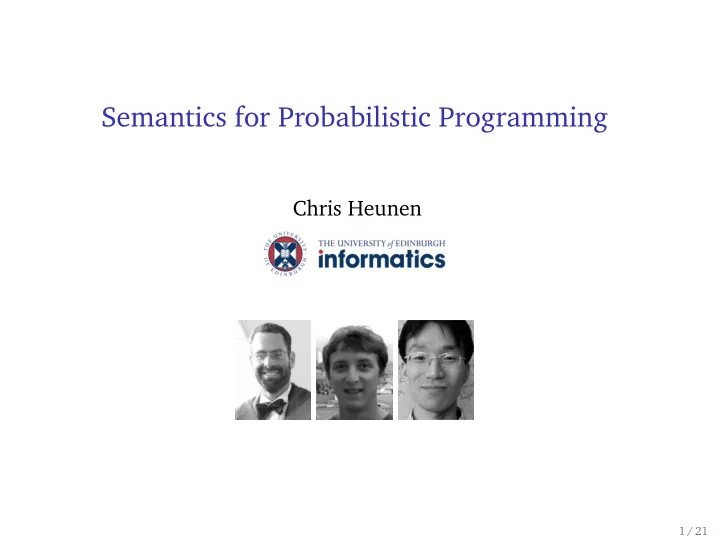
Semantics for Probabilistic Programming Chris Heunen 1 / 21 Bayes - PowerPoint PPT Presentation

Semantics for Probabilistic Programming Chris Heunen 1 / 21

Bayes’ law P ( A | B ) = P ( B | A ) × P ( A ) P ( B ) 2 / 21

Bayes’ law P ( A | B ) = P ( B | A ) × P ( A ) P ( B ) Bayesian reasoning: ◮ predict future, based on model and prior evidence ◮ infer causes, based on model and posterior evidence ◮ learn better model, based on prior model and evidence 2 / 21

Bayesian networks 3 / 21

Bayesian inference 4 / 21

Linear regression 5 / 21

Probabilistic programming P ( A | B ) ∝ P ( B | A ) × P ( A ) posterior ∝ likelihood × prior functional programming + observe + sample 6 / 21

Probabilistic programming P ( A | B ) ∝ P ( B | A ) × P ( A ) posterior ∝ likelihood × prior functional programming + observe + sample 6 / 21

Linear regression (defquery Bayesian-linear-regression (let [f (let [s (sample (normal 0.0 3.0)) b (sample (normal 0.0 3.0))] (fn [x] (+ (* s x) b)))] (observe (normal (f 1.0) 0.5) 2.5) (observe (normal (f 2.0) 0.5) 3.8) (observe (normal (f 3.0) 0.5) 4.5) (observe (normal (f 4.0) 0.5) 6.2) (observe (normal (f 5.0) 0.5) 8.0) (predict :f f))) 7 / 21

Linear regression 8 / 21

Linear regression 9 / 21

Measure theory Impossible to sample 0 . 5 from standard normal distribution But sample in interval ( 0 , 1 ) with probability around 0 . 34 10 / 21

Measure theory Impossible to sample 0 . 5 from standard normal distribution But sample in interval ( 0 , 1 ) with probability around 0 . 34 A measurable space is a set X with a family Σ X of subsets that is closed under countable unions and complements A (probability) measure on X is a function p : Σ X → [ 0 , ∞ ] that satisfies p ( � U n ) = � p ( U n ) (and has p ( X ) = 1) 10 / 21

Measure theory Impossible to sample 0 . 5 from standard normal distribution But sample in interval ( 0 , 1 ) with probability around 0 . 34 A measurable space is a set X with a family Σ X of subsets that is closed under countable unions and complements A (probability) measure on X is a function p : Σ X → [ 0 , ∞ ] that satisfies p ( � U n ) = � p ( U n ) (and has p ( X ) = 1) A function f : X → Y is measurable if f − 1 ( U ) ∈ Σ X for U ∈ Σ Y A random variable is a measurable function R → X 10 / 21

Function types Z × X f × id X ˆ f [ X → Y ] × X Y ev 11 / 21

Function types Z × X f × id X ˆ f [ X → Y ] × X Y ev [ R → R ] cannot be a measurable space! 11 / 21

Quasi-Borel spaces A quasi-Borel space is a set X together with M X ⊆ [ R → X ] satisfying: ◮ α ◦ f ∈ M X if α ∈ M X and f : R → R is measurable ◮ α ∈ M X if α : R → X is constant ◮ if R = � n ∈ N S n , with each set S n Borel, and α 1 , α 2 , . . . ∈ M X , then β is in M X , where β ( r ) = α n ( r ) for r ∈ S n 12 / 21

Quasi-Borel spaces A quasi-Borel space is a set X together with M X ⊆ [ R → X ] satisfying: ◮ α ◦ f ∈ M X if α ∈ M X and f : R → R is measurable ◮ α ∈ M X if α : R → X is constant ◮ if R = � n ∈ N S n , with each set S n Borel, and α 1 , α 2 , . . . ∈ M X , then β is in M X , where β ( r ) = α n ( r ) for r ∈ S n A morphism is a function f : X → Y with f ◦ α ∈ M Y if α ∈ M X ◮ has product types ◮ has countable sum types ◮ has function types! M [ X → Y ] = { α : R → [ X → Y ] | ˆ α : R × X → Y morphism } 12 / 21

Distribution types A measure on a quasi-Borel space ( X , M X ) consists of ◮ α ∈ M X and ◮ a probability measure µ on R Two measures are identified when they induce the same µ ( α − 1 ( − )) 13 / 21

Distribution types A measure on a quasi-Borel space ( X , M X ) consists of ◮ α ∈ M X and ◮ a probability measure µ on R Two measures are identified when they induce the same µ ( α − 1 ( − )) Gives monad ◮ P ( X , M X ) = { ( α, µ ) measure on ( X , M X } / ∼ ◮ return x = [ λ r . x , µ ] ∼ for arbitrary µ ◮ bind uses integral � � f d ( α, µ ) := ( f ◦ α ) d µ if f : ( X , M X ) → R for distribution types 13 / 21

Example: facts about distributions � � let x = sample(gauss(0.0,1.0)) = � sample(bern(0.5)) � in return (x<0) 14 / 21

Example: importance sampling � � sample(exp(2)) � let x = sample(gauss(0,1))) � = observe(exp-pdf(2,x)/gauss-pdf(0,1,x)); return x 15 / 21

Example: conjugate priors � let x = sample(beta(1,1)) � � observe(bern(0.5), true); � = in observe(bern(x), true); let x = sample(beta(2,1)) return x in return x 16 / 21

Linear regression (defquery Bayesian-linear-regression Prior: (let [f (let [s (sample (normal 0.0 3.0)) b (sample (normal 0.0 3.0))] (fn [x] (+ (* s x) b)))] Likelihood: (observe (normal (f 1.0) 0.5) 2.5) (observe (normal (f 2.0) 0.5) 3.8) (observe (normal (f 3.0) 0.5) 4.5) (observe (normal (f 4.0) 0.5) 6.2) (observe (normal (f 5.0) 0.5) 8.0) Posterior: (predict :f f))) 17 / 21

Linear regression: prior Define a prior measure on [ R → R ] � (let [f (let [s (sample (normal 0.0 3.0)) � b (sample (normal 0.0 3.0))] (fn [x] (+ (* s x) b)))] = [ α, ν ⊗ ν ] ∼ ∈ P ([ R → R ]) where ν is normal distribution, mean 0 and standard deviation 3, and α : R × R → [ R → R ] is ( s , b ) �→ λ r . sr + b 18 / 21

Linear regression: likelihood Define likelihood of observations (with some noise) � � (observe (normal (f 1.0) 0.5) 2.5) � � (observe (normal (f 2.0) 0.5) 3.8) � � � � (observe (normal (f 3.0) 0.5) 4.5) � � (observe (normal (f 4.0) 0.5) 6.2) (observe (normal (f 5.0) 0.5) 8.0) = d ( f ( 1 ) , 2 . 5 ) · d ( f ( 2 ) , 3 . 8 ) · d ( f ( 3 ) , 4 . 5 ) · d ( f ( 4 ) , 6 . 2 ) · d ( f ( 5 ) , 8 . 0 ) where f free variable of type [ R → R ] , and d : R 2 → [ 0 , ∞ ) is density of normal distribution with standard deviation 0.5 � 2 /π exp ( − 2 ( x − µ ) 2 ) d ( µ, x ) = 19 / 21

Linear regression: Posterior Normalise combined prior and likelihood � (predict :f f))) � ∈ P ([ R → R ]) 20 / 21

Want more? ◮ “ Semantics for probabilistic programming: higher-order functions, continuous distributions, and soft constraints ” LiCS 2016 ◮ “ A convenient category for higher-order probability theory ” arXiv:1701.02547 21 / 21