Segmentation Professor Fei Fei Li Stanford Vision Lab 1 19 Apr 11 - PowerPoint PPT Presentation

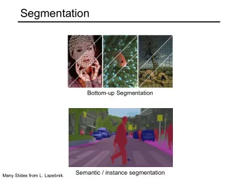
Segmentation Professor Fei ‐ Fei Li Stanford Vision Lab 1 19 ‐ Apr ‐ 11 Lecture 8 - Fei-Fei Li

Image Segmentation • Goal: identify groups of pixels that go together 2 19 ‐ Apr ‐ 11 Lecture 8 - Fei-Fei Li

Success Story 3 19 ‐ Apr ‐ 11 Fei-Fei Li Lecture 8 -

Gestalt Theory • Gestalt: whole or group – Whole is greater than sum of its parts – Relationships among parts can yield new properties/features • Psychologists identified series of factors that predispose set of elements to be grouped (by human visual system) “I stand at the window and see a house, trees, sky. Theoretically I might say there were 327 brightnesses and nuances of colour. Do I have "327"? No. I have sky, house, and trees.” Max Wertheimer (1880-1943) Untersuchungen zur Lehre von der Gestalt, Psychologische Forschung , Vol. 4, pp. 301-350, 1923 http://psy.ed.asu.edu/~classics/Wertheimer/Forms/forms.htm 4 19 ‐ Apr ‐ 11 Lecture 8 - Fei-Fei Li

Gestalt Factors These factors make intuitive sense, but are very difficult to translate into algorithms. • 5 19 ‐ Apr ‐ 11 Lecture 8 - Fei-Fei Li

K ‐ Means Clustering • Basic idea: randomly initialize the k cluster centers, and iterate between the two steps we just saw. Randomly initialize the cluster centers, c 1 , ..., c K 1. Given cluster centers, determine points in each cluster 2. • For each point p, find the closest c i . Put p into cluster i Given points in each cluster, solve for c i 3. • Set c i to be the mean of points in cluster i If c i have changed, repeat Step 2 4. 6 19 ‐ Apr ‐ 11 Lecture 8 - Fei-Fei Li

Expectation Maximization (EM) • Goal Find blob parameters θ that maximize the likelihood function: – • Approach: E ‐ step: given current guess of blobs, compute ownership of each point 1. M ‐ step: given ownership probabilities, update blobs to maximize likelihood 2. function Repeat until convergence 3. 7 19 ‐ Apr ‐ 11 Lecture 8 - Fei-Fei Li

Mean ‐ Shift Algorithm • Iterative Mode Search Initialize random seed, and window W 1. Calculate center of gravity (the “mean”) of W: 2. Shift the search window to the mean 3. Repeat Step 2 until convergence 4. 8 19 ‐ Apr ‐ 11 Lecture 8 - Fei-Fei Li

Mean ‐ Shift Segmentation Find features (color, gradients, texture, etc) • • Initialize windows at individual pixel locations • Perform mean shift for each window until convergence • Merge windows that end up near the same “peak” or mode 9 19 ‐ Apr ‐ 11 Lecture 8 - Fei-Fei Li

Back to the Image Segmentation Problem… • Goal: identify groups of pixels that go together • Up to now, we have focused on ways to group pixels into image segments based on their appearance… – Segmentation as clustering. • We also want to enforce region constraints. – Spatial consistency – Smooth borders 10 19 ‐ Apr ‐ 11 Lecture 8 - Fei-Fei Li

What we will learn today? • Graph theoretic segmentation – Normalized Cuts – Using texture features • Segmentation as Energy Minimization – Markov Random Fields – Graph cuts for image segmentation – Applications 11 19 ‐ Apr ‐ 11 Lecture 8 - Fei-Fei Li

What we will learn today? • Graph theoretic segmentation – Normalized Cuts – Using texture features • Segmentation as Energy Minimization – Markov Random Fields – Graph cuts for image segmentation – Applications 12 19 ‐ Apr ‐ 11 Lecture 8 - Fei-Fei Li

Images as Graphs q w pq w p • Fully ‐ connected graph – Node (vertex) for every pixel – Link between every pair of pixels, (p,q) – Affinity weight w pq for each link (edge) • w pq measures similarity • Similarity is inversely proportional to difference (in color and position…) S lide credit: S teve S eitz 13 19 ‐ Apr ‐ 11 Lecture 8 - Fei-Fei Li

Segmentation by Graph Cuts w A B C • Break Graph into Segments – Delete links that cross between segments – Easiest to break links that have low similarity (low weight) • Similar pixels should be in the same segments • Dissimilar pixels should be in different segments S lide credit: S teve S eitz 14 19 ‐ Apr ‐ 11 Lecture 8 - Fei-Fei Li

Measuring Affinity { } 2 = − − aff x y x y 1 ( , ) exp • Distance σ 2 2 d { } 2 = − − • Intensity aff x y I x I y 1 ( , ) exp ( ) ( ) σ 2 2 d { } ( ) 2 = − aff x y dist c x c y • Color ( , ) exp 1 ( ), ( ) σ 2 2 d (some suitable color space distance) ource: Forsyth & Ponce { } 2 = − − aff x y f x f y • Texture ( , ) exp 1 ( ) ( ) σ 2 2 d (vectors of filter outputs) S 15 19 ‐ Apr ‐ 11 Lecture 8 - Fei-Fei Li

Scale Affects Affinity • Small σ : group only nearby points • Large σ : group far ‐ away points Small σ Medium σ Large σ S lide credit: S vetlana Lazebnik 16 19 ‐ Apr ‐ 11 Lecture 8 - Fei-Fei Li

Graph Cut: using Eigenvalues • Extract a single good cluster – Where elements have high affinity values with each other points Lecture 8 - Fei-Fei Li

Graph Cut: using Eigenvalues matrix • Extract a single good cluster Eigenvector associated w/ the largest eigenvalue points Fei-Fei Li Lecture 8 -

Graph Cut: using Eigenvalues • Extract a single good cluster • Extract weights for a set of clusters Eigenvector associated Eigenvectors associated with other eigenvalues w/ the largest eigenvalue Lecture 8 - Fei-Fei Li

Graph Cut: using Eigenvalues (effect of the scaling factor) Fei-Fei Li Lecture 8 -

Fei-Fei Li Lecture 8 -

Graph Cut B A • Set of edges whose removal makes a graph disconnected • Cost of a cut ∑ = cut A B w ( , ) – Sum of weights of cut edges: p q , ∈ ∈ p A q B , • A graph cut gives us a segmentation – What is a “good” graph cut and how do we find one? S lide credit: S teve S eitz 22 19 ‐ Apr ‐ 11 Lecture 8 - Fei-Fei Li

Graph Cut Here, the cut is nicely defined by the block-diagonal structure of the affinity matrix. ⇒ How can this be generalized? Image S ource: Forsyth & Ponce 23 19 ‐ Apr ‐ 11 Lecture 8 - Fei-Fei Li

Minimum Cut We can do segmentation by finding the minimum cut in a graph • – a minimum cut of a graph is a cut whose cutset has the smallest number of elements (unweighted case) or smallest sum of weights possible. – Efficient algorithms exist for doing this • Drawback: Weight of cut proportional to number of edges in the cut – hafique – Minimum cut tends to cut off very small, isolated components lide credit: Khurram Hassan-S Cuts with lesser weight than the ideal cut Ideal Cut S 24 19 ‐ Apr ‐ 11 Lecture 8 - Fei-Fei Li

Normalized Cut (NCut) • A minimum cut penalizes large segments • This can be fixed by normalizing for size of segments • The normalized cut cost is: cut A B cut A B ( , ) ( , ) + assoc A V assoc B V ( , ) ( , ) assoc ( A , V ) = sum of weights of all edges in V that touch A • The exact solution is NP ‐ hard but an approximation can be computed by solving a generalized eigenvalue problem. J. Shi and J. Malik. Normalized cuts and image segmentation. PAMI 2000 25 19 ‐ Apr ‐ 11 Lecture 8 - Fei-Fei Li

Interpretation as a Dynamical System eitz teve S • Treat the links as springs and shake the system – Elasticity proportional to cost lide credit: S – Vibration “modes” correspond to segments • Can compute these by solving a generalized eigenvector problem S 26 19 ‐ Apr ‐ 11 Lecture 8 - Fei-Fei Li

NCuts as a Generalized Eigenvector Problem • Definitions = W W i j w : ( , ) ; the affinity matrix, i j , ∑ = D D i i W i j : ( , ) ( , ); the diag. matrix, j − = ⇔ ∈ N x x i i A : {1, 1} , ( ) 1 . a vector in • Rewriting Normalized Cut in matrix form: cut cut (A,B) (A,B) = + NCut (A,B) assoc assoc (A,V) (B,V) ∑ D i i ( , ) + − + − − − T T x D W x x D W x (1 ) ( )(1 ) (1 ) ( )(1 ) > x = + = 0 k ; i ∑ − T T k D k D D i i 1 1 (1 )1 1 ( , ) i = ... S lide credit: Jitendra Malik 27 19 ‐ Apr ‐ 11 Lecture 8 - Fei-Fei Li

Some More Math… lide credit: Jitendra Malik S 28 19 ‐ Apr ‐ 11 Lecture 8 - Fei-Fei Li

NCuts as a Generalized Eigenvalue Problem After simplification, we get • − T y D W y ( ) This is hard, = ∈ − = T NCut A B y b y D ( , ) , with {1, }, 1 0. i as y is discrete! T y Dy • This is a Rayleigh Quotient – Solution given by the “generalized” eigenvalue problem – Solved by converting to standard eigenvalue problem 1 1 1 − − − = = D (D W)D z λ z where z D y , 2 2 2 Relaxation: continuous y . • Subtleties – Optimal solution is second smallest eigenvector – Gives continuous result—must convert into discrete values of y S lide credit: Alyosha Efros 29 19 ‐ Apr ‐ 11 Lecture 8 - Fei-Fei Li

NCuts Example Smallest eigenvectors NCuts segments Image source: S hi & Malik 30 19 ‐ Apr ‐ 11 Lecture 8 - Fei-Fei Li