Searching Complexity of Binary Search Hans-Joachim Bckenhauer and - PowerPoint PPT Presentation

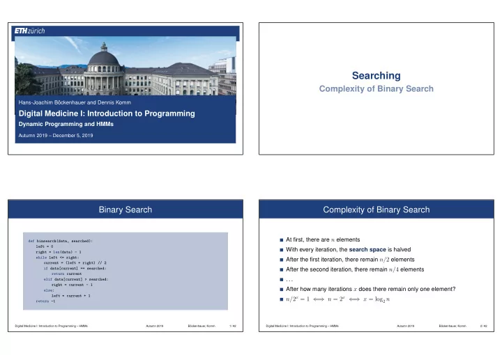
Searching Complexity of Binary Search Hans-Joachim Böckenhauer and Dennis Komm Digital Medicine I: Introduction to Programming Dynamic Programming and HMMs Autumn 2019 – December 5, 2019 Binary Search Complexity of Binary Search At first, there are n elements def binsearch(data, searched): left = 0 With every iteration, the search space is halved right = len(data) - 1 while left <= right: After the first iteration, there remain n/ 2 elements current = (left + right) // 2 After the second iteration, there remain n/ 4 elements if data[current] == searched: return current . . . elif data[current] > searched: right = current - 1 After how many iterations x does there remain only one element? else: left = current + 1 n/ 2 x = 1 ⇐ ⇒ n = 2 x ⇐ ⇒ x = log 2 n return -1 Digital Medicine I: Introduction to Programming – HMMs Autumn 2019 Böckenhauer, Komm 1 / 42 Digital Medicine I: Introduction to Programming – HMMs Autumn 2019 Böckenhauer, Komm 2 / 42

Complexity of Binary Search Complexity of Binary Search 100 Linear search 80 We again use a variable counter to count the comparisons Comparisons Algorithm is executed on sorted lists with values 1 to n 60 The value of n grows by 1 with every iteration 40 Initially, n is 1, at the end 1 000 000 20 The first element 1 is always sought Binary search Binary search Results are stored in a list and plotted using matplotlib 0 10 20 30 40 50 60 70 80 90 100 Input length n Digital Medicine I: Introduction to Programming – HMMs Autumn 2019 Böckenhauer, Komm 3 / 42 Digital Medicine I: Introduction to Programming – HMMs Autumn 2019 Böckenhauer, Komm 4 / 42 Complexity of Binary Search Complexity of Binary Search Worst Case What happens if data is unsorted? values = [] data = [1] Linear search always works for unsorted lists and is in O ( n ) Sorting can pay off for multiple searches Sorting is in O ( n log n ) and is therefore slower than linear search for i in range(1, 1000001): data.append(data[-1] + 1) Binary search is in O (log n ) and is consequently much faster than linear values.append(binsearch(data, 1)) search Add element that is larger by 1 than plt.plot(values, color="red") When does sorting pay off? plt.show() the currently last If more than log n searches are made Digital Medicine I: Introduction to Programming – HMMs Autumn 2019 Böckenhauer, Komm 5 / 42 Digital Medicine I: Introduction to Programming – HMMs Autumn 2019 Böckenhauer, Komm 6 / 42

Observing a Bacterial Culture How does a bacterial culture change over time? A Question Nutrient solution in changing environment (Temperature increase, addition of chemicals, . . . ) from Medical Research We want to study: When are bacteria sick, when healthy? If healthy, some protein is produced Altered bacteria DNA (Fluorescence marker, GFP) Observe fluorescence level over time Digital Medicine I: Introduction to Programming – HMMs Autumn 2019 Böckenhauer, Komm 7 / 42 Observing a Bacterial Culture Time in minutes 60 140 250 300 390 450 550 600 a Observation Hidden Markov Models b The Unfair Casino 120 Elowitz, Leibler, 2000, Nature 403 For the fluorescence level, we observe Low , Medium , Medium , High , Medium , High , Medium , High What follows for the health condition of the bacteria? Digital Medicine I: Introduction to Programming – HMMs Autumn 2019 Böckenhauer, Komm 8 / 42

The Unfair Casino Markov Model for the Unfair Casino (All results with probability 1 A fair die 6 ) with probability 1 19 19 An unfair (loaded) die (Result 2 ) Start 20 20 (Probability 1 At beginning one is chosen 2 ) 1 1 2 2 (Probability 1 After each roll the die can be (secretly) switched 20 ) Fair Unfair 1 Markov Model Prob ( ) = 0 . 16 Prob ( ) = 0 . 1 20 Prob ( ) = 0 . 16 Prob ( ) = 0 . 1 State: Die currently used Prob ( ) = 0 . 16 Prob ( ) = 0 . 1 Prob ( ) = 0 . 16 Prob ( ) = 0 . 1 1 Transition probability: Prob ( ) = 0 . 16 Prob ( ) = 0 . 1 20 Prob ( ) = 0 . 16 Prob ( ) = 0 . 5 Probability to switch the die Emission probability: Probability to observe concrete number; depending on the current state Digital Medicine I: Introduction to Programming – HMMs Autumn 2019 Böckenhauer, Komm 9 / 42 Digital Medicine I: Introduction to Programming – HMMs Autumn 2019 Böckenhauer, Komm 10 / 42 Probability of a Concrete Output Probability of a Concrete Output Consider the first 1. Event A = “The unfair die is chosen at the beginning” Suppose we observe , , , 2. Event B = “The is rolled” Moreover, we know that first the unfair die was used twice, and then the fair one was used twice Prob ( The unfair die is chosen at the beginning and is rolled ) This is a fixed walk through our Markov model = Prob ( A and B ) = Prob ( A ) · Prob ( B under the condition A ) How large is the probability? = Prob ( A ) · Prob ( B | A ) = 1 2 · 1 2 Digital Medicine I: Introduction to Programming – HMMs Autumn 2019 Böckenhauer, Komm 11 / 42 Digital Medicine I: Introduction to Programming – HMMs Autumn 2019 Böckenhauer, Komm 12 / 42

Probability of a Concrete Output Probability of a Concrete Output We can continue in this fashion for , , , Hidden Markov Model (HMM) But what happens if we only observe the outputs? 2 · 1 1 2 · 19 20 · 1 2 · 1 20 · 1 6 · 19 20 · 1 Suppose we observe , , , , 6 What is the most probable walk? For three numbers, the unfair die is “better” For two numbers, the fair one is “better” 361 Is it worth to switch the die? 2 304 000 Digital Medicine I: Introduction to Programming – HMMs Autumn 2019 Böckenhauer, Komm 13 / 42 Digital Medicine I: Introduction to Programming – HMMs Autumn 2019 Böckenhauer, Komm 14 / 42 Probability that the die is not switched Probability that the unfair die is chosen at the beginning Probability that then a Total probability Probability that then a Probability that the die is switched Probability that then a Probability that the die is not switched Probability that another is rolled again is rolled is rolled again is rolled Probability of a Concrete Output Number of possible walks for n rolls is 2 n For 300 rolls this is more than Hidden Markov Models 10 90 Dynamic Programming Do we really need to try them all? No ➯ Dynamic programming Digital Medicine I: Introduction to Programming – HMMs Autumn 2019 Böckenhauer, Komm 15 / 42

Dynamic Programming Viterbi Algorithm X 1 X 2 X 3 X 4 X 5 X 6 X 7 Idea Solution for complete input is put together from solutions for subproblems, “fair” starting with smallest subproblems “unfair” Problem: Find suitable subproblems Viterbi Algorithm (Viterbi, 1967) Suppose shaded cells are already filled out All most probable walks for prefixes of the given sequence that end in Most probable walks of length 3 are known particular state are partial solutions (e.g., walk that ends with observation X 3 is: “unfair, ” “fair, ” “fair”) Compute most probable walks for larger prefixes from most probable Compute such a walk of length 4 ending in “fair” walks for smaller ones Extend known walks and take more probable one Digital Medicine I: Introduction to Programming – HMMs Autumn 2019 Böckenhauer, Komm 16 / 42 Digital Medicine I: Introduction to Programming – HMMs Autumn 2019 Böckenhauer, Komm 17 / 42 Viterbi Algorithm Observe sequence , , , , Create table Store which walk is the most probable so far Hidden Markov Models for Bacterial Culture 2 · 1 1 1 19 361 6859 6859 “fair” Probability of the most 12 6 1440 172800 20736000 76800000 � 1 19 12 · 19 20 , 1 4 · 1 probable walk of length 2 � max 240 19 Probability that is 20 ending in “fair” 2 · 1 1 1 19 361 6859 130321 “unfair” · observed and the state is 1440 4 2 800 16000 640000 25600000 “fair” Probability that 1 Most probable walk: only unfair die is observed in “fair” 6 Digital Medicine I: Introduction to Programming – HMMs Autumn 2019 Böckenhauer, Komm 18 / 42

Observing a Bacterial Culture Observing a Bacterial Culture Bacterium can be in one of three states: Time in minutes 1. Healthy 60 140 250 300 390 450 550 600 a Observation 2. OK 3. Sick b DNA is changed so that bacteria fluoresce; the more, the more healthy they are. 120 Elowitz, Leibler, 2000, Nature 403 Fluorescence level: For the fluorescence level, we observe 1. High Low , Medium , Medium , High , Medium , High , Medium , High 2. Medium What follows for the health condition of the bacteria? 3. Low Digital Medicine I: Introduction to Programming – HMMs Autumn 2019 Böckenhauer, Komm 19 / 42 Digital Medicine I: Introduction to Programming – HMMs Autumn 2019 Böckenhauer, Komm 20 / 42 Observing a Bacterial Culture Observing a Bacterial Culture Emission probabilities (empirical results) Transition probabilities (empirical results) Prob ( High ) = 0 . 5 0 . 6 1. Healthy: Prob ( Medium ) = 0 . 3 OK Prob ( High ) = 0 . 2 Prob ( Low ) = 0 . 2 Prob ( Medium ) = 0 . 6 Prob ( Low ) = 0 . 2 0 . 3 0 . 2 Prob ( High ) = 0 . 2 2. OK: Prob ( Medium ) = 0 . 6 Prob ( Low ) = 0 . 2 0 . 2 0 . 4 Healthy Sick Prob ( High ) = 0 . 2 Prob ( High ) = 0 . 5 Prob ( High ) = 0 . 2 0 . 4 0 . 6 Prob ( Medium ) = 0 . 3 0 . 3 Prob ( Medium ) = 0 . 3 3. Sick: Prob ( Medium ) = 0 . 3 Prob ( Low ) = 0 . 2 Prob ( Low ) = 0 . 5 Prob ( Low ) = 0 . 5 Digital Medicine I: Introduction to Programming – HMMs Autumn 2019 Böckenhauer, Komm 21 / 42 Digital Medicine I: Introduction to Programming – HMMs Autumn 2019 Böckenhauer, Komm 22 / 42