Sampling Michel Bierlaire Transport and Mobility Laboratory School - PowerPoint PPT Presentation
Sampling Michel Bierlaire Transport and Mobility Laboratory School of Architecture, Civil and Environmental Engineering Ecole Polytechnique F ed erale de Lausanne M. Bierlaire (TRANSP-OR ENAC EPFL) Sampling 1 / 53 Outline Outline
Sampling Michel Bierlaire Transport and Mobility Laboratory School of Architecture, Civil and Environmental Engineering Ecole Polytechnique F´ ed´ erale de Lausanne M. Bierlaire (TRANSP-OR ENAC EPFL) Sampling 1 / 53
Outline Outline Introduction 1 Sampling strategies 2 Estimation: maximum likelihood 3 Conditional maximum likelihood 4 M. Bierlaire (TRANSP-OR ENAC EPFL) Sampling 2 / 53
Introduction Introduction Sampling strategy Does the sample perfectly reflect the population? Is it desirable to perform random sampling? How will other sampling strategies affect the model estimates? What are the specific implications for discrete choice? M. Bierlaire (TRANSP-OR ENAC EPFL) Sampling 3 / 53
Introduction Introduction Until now... ... we have assumed that x is fixed: P ( i | x ; β ) . When we draw a sample, actually we draw both i and x . We need to write the joint probability of i and x : f ( i , x | β ) = P ( i | x ; β ) f ( x ) . Depending on how the sample is drawn, this may impact the estimator. M. Bierlaire (TRANSP-OR ENAC EPFL) Sampling 4 / 53
Introduction Types of variables Exogenous/independent variables (denoted by x ) age, gender, income, prices Not modeled, treated as given in the population May be subject to what if policy manipulations Endogenous/dependent variable (denoted by i ) Choice Modeling assumption Causality: P ( i | x ; θ ) M. Bierlaire (TRANSP-OR ENAC EPFL) Sampling 5 / 53
Introduction Types of variables The nature of a variable depends on the application Example: residential location Endogenous in a house choice study Exogenous in a study about transport mode choice to work Meaningful modeling assumption A model P ( i | x ; θ ) may fit the data and describe correlation between i and x without being a causal model. Example: P(crime | temp) and P(temp | crime). Important Critical to identify the causal relationship and, therefore, exogenous and endogenous variables. M. Bierlaire (TRANSP-OR ENAC EPFL) Sampling 6 / 53
Sampling strategies Outline Introduction 1 Sampling strategies 2 Estimation: maximum likelihood 3 Exogenous sample maximum likelihood Conditional maximum likelihood 4 Logit and choice-based sample MEV and choice-based sample M. Bierlaire (TRANSP-OR ENAC EPFL) Sampling 7 / 53
Sampling strategies Sampling strategies Simple Random Sample (SRS) Probability of being drawn: R R is identical for each individual Convenient for model estimation and forecasting Very difficult to conduct in practice Exogenously Stratified Sample (XSS) Probability of being drawn: R ( x ) R ( x ) varies with variables other than i May also vary with variables outside the model Examples: oversampling of workers for mode choice oversampling of women for baby food choice undersampling of old people for choice of a retirement plan M. Bierlaire (TRANSP-OR ENAC EPFL) Sampling 8 / 53
Sampling strategies Sampling strategies Endogenously Stratified Sample (ESS) Probability of being drawn: R ( i , x ) R ( i , x ) varies with dependent variables Examples: oversampling of bus riders products with small market shares: if SRS, likely that no observation of i in the sample (ex: Ferrari) oversampling of current customers M. Bierlaire (TRANSP-OR ENAC EPFL) Sampling 9 / 53
Sampling strategies Sampling strategies Pure choice-based sampling Probability of being drawn: R ( i ) R ( i ) varies only with dependent variables Special case of ESS M. Bierlaire (TRANSP-OR ENAC EPFL) Sampling 10 / 53
Sampling strategies Sampling strategies Stratified sampling In practice, groups are defined, and individuals are sampled randomly within each group. Example: mode choice Let’s consider each sampling scheme on the following example: Exogenous variable: travel time by car Endogenous variable: transportation mode M. Bierlaire (TRANSP-OR ENAC EPFL) Sampling 11 / 53
Sampling strategies Sampling strategies Simple Random Sampling (SRS): one group = population Drive alone Carpooling Transit Travel ≤ 15 time > 15, ≤ 30 by car > 30 M. Bierlaire (TRANSP-OR ENAC EPFL) Sampling 12 / 53
Sampling strategies Sampling strategies Exogenously Stratified Sample (XSS) Drive alone Carpooling Transit Travel ≤ 15 time > 15, ≤ 30 by car > 30 M. Bierlaire (TRANSP-OR ENAC EPFL) Sampling 13 / 53
Sampling strategies Sampling strategies Pure choice-based sampling Drive alone Carpooling Transit Travel ≤ 15 time > 15, ≤ 30 by car > 30 M. Bierlaire (TRANSP-OR ENAC EPFL) Sampling 14 / 53
Sampling strategies Sampling strategies Endogenously Stratified Sample (ESS) Drive alone Carpooling Transit Travel ≤ 15 time > 15, ≤ 30 by car > 30 M. Bierlaire (TRANSP-OR ENAC EPFL) Sampling 15 / 53
Sampling strategies Sampling strategies If ( i , x ) belongs to group g , we can write R ( i , x ) = H g N s W g N where H g is the fraction of the group corresponding to ( i , x ) in the sample W g is the fraction of the group corresponding to ( i , x ) in the population N s is the sample size N is the population size M. Bierlaire (TRANSP-OR ENAC EPFL) Sampling 16 / 53
Sampling strategies Sampling strategies Calculation H g and N s are decided by the analyst W g can be expressed as � � p ( x ) dx W g = P ( i | x , θ ) x i ∈C g which is a function of θ . M. Bierlaire (TRANSP-OR ENAC EPFL) Sampling 17 / 53
Sampling strategies Sampling strategies Simplification If group g contains all alternatives, then � P ( i | x , θ ) = 1 i ∈C g � and W g = x ∈ g p ( x ) dx does not depend on θ This can happen only if groups are not defined based on the alternatives. M. Bierlaire (TRANSP-OR ENAC EPFL) Sampling 18 / 53
Sampling strategies Illustration Population i=0 i=1 x=0 300000 100000 400000 40% x=1 510000 90000 600000 60% 810000 190000 1000000 81% 19% Simple random sample (SRS) x=0 300 100 400 40% x=0 1/1000 1/1000 x=1 510 90 600 60% x=1 1/1000 1/1000 810 190 1000 81% 19% M. Bierlaire (TRANSP-OR ENAC EPFL) Sampling 19 / 53
Sampling strategies Illustration Population i=0 i=1 x=0 300000 100000 400000 40% x=1 510000 90000 600000 60% 810000 190000 1000000 81% 19% Exogenously Stratified Sample (XSS) x=0 187.5 62.5 250 25% x=0 1/1600 1/1600 x=1 637.5 112.5 750 75% x=1 1/800 1/800 825 175 1000 83% 18% M. Bierlaire (TRANSP-OR ENAC EPFL) Sampling 20 / 53
Sampling strategies Illustration Population i=0 i=1 x=0 300000 100000 400000 40% x=1 510000 90000 600000 60% 810000 190000 1000000 81% 19% Choice based stratified sampling x=0 252.1 168.1 420.2 42% x=0 1/1190 1/595 x=1 428.6 151.3 579.9 58% x=1 1/1190 1/595 680.7 319.3 1000 68% 32% M. Bierlaire (TRANSP-OR ENAC EPFL) Sampling 21 / 53
Estimation: maximum likelihood Outline Introduction 1 Sampling strategies 2 Estimation: maximum likelihood 3 Exogenous sample maximum likelihood Conditional maximum likelihood 4 Logit and choice-based sample MEV and choice-based sample M. Bierlaire (TRANSP-OR ENAC EPFL) Sampling 22 / 53
Estimation: maximum likelihood Estimation Define s n as the event of individual n being in the sample Maximum Likelihood N � max L ( θ ) = ln f ( i n , x n | s n ; θ ) θ n =1 The joint probability for an individual to be in the sample ( s n ) be exposed to exogenous variables x n choose the observed alternative ( i n ) is denoted f ( i n , x n , s n ; θ ) M. Bierlaire (TRANSP-OR ENAC EPFL) Sampling 23 / 53
Estimation: maximum likelihood Estimation Bayes theorem f ( i n , x n , s n ; θ ) = f ( i n , x n | s n ; θ ) f ( s n ; θ ) = f ( s n | i n , x n ; θ ) f ( i n | x n ; θ ) p ( x n ) . f ( i n , x n | s n ; θ ) f ( s n ; θ ) = f ( s n | i n , x n ; θ ) f ( i n | x n ; θ ) p ( x n ) f ( i n , x n | s n ; θ ): term for the ML f ( s n ; θ ) = � � j ∈C f ( s n | j , z ; θ ) f ( j | z ; θ ) f ( z ) z f ( s n | i n , x n ; θ ): probability to be sampled, that is R ( i n , x n ; θ ) f ( i n | x n ; θ ): choice model P ( i n | x n ; θ ) Contribution to the likelihood function R ( i n , x n ; θ ) P ( i n | x n ; θ ) p ( x n ) f ( i n , x n | s n ; θ ) = � � j ∈C R ( j , z ; θ ) P ( j | z ; θ ) p ( z ) z M. Bierlaire (TRANSP-OR ENAC EPFL) Sampling 24 / 53
Estimation: maximum likelihood Estimation Contribution to the likelihood function R ( i n , x n ; θ ) P ( i n | x n ; θ ) p ( x n ) f ( i n , x n | s n ; θ ) = � � j ∈C R ( j , z ; θ ) P ( j | z ; θ ) p ( z ) z In general, impossible to handle Namely, p ( z ) is usually not available In practice It does simplify when the sampling is exogenous If not, we use Conditional Maximum Likelihood instead. Case of logit Case of MEV Other models M. Bierlaire (TRANSP-OR ENAC EPFL) Sampling 25 / 53
Estimation: maximum likelihood Exogenous sample maximum likelihood Exogenous Sample Maximum Likelihood If the sample is simple or exogenous R ( i , x ; θ ) = R ( x ) ∀ i , θ Contribution to the likelihood function R ( i n , x n ; θ ) P ( i n | x n ; θ ) p ( x n ) f ( i n , x n | s n ; θ ) = � � j ∈C R ( j , z ; θ ) P ( j | z ; θ ) p ( z ) z R ( x n ) P ( i n | x n ; θ ) p ( x n ) = � � j ∈C R ( z ) P ( j | z ; θ ) p ( z ) z R ( x n ) P ( i n | x n ; θ ) p ( x n ) = � z R ( z ) p ( z ) � j ∈C P ( j | z ; θ ) R ( x n ) P ( i n | x n ; θ ) p ( x n ) = � z R ( z ) p ( z ) M. Bierlaire (TRANSP-OR ENAC EPFL) Sampling 26 / 53
Recommend
More recommend
Explore More Topics
Stay informed with curated content and fresh updates.


![CS786 Lecture 13: May 14, 2012 Sampling techniques [KF Chapter 12] CS786 P. Poupart 2012 1](https://c.sambuz.com/696755/cs786-lecture-13-may-14-2012-s.webp)
