Sampling and Inference Sampling and Inference The Quality of Data and - PowerPoint PPT Presentation
Sampling and Inference Sampling and Inference The Quality of Data and Measures 2012 1 Why do we sample? Cost/ benefit benefit Benefit Benefit (precision) Cost (h (hassle factor) l f t ) N 2 Effects of samples Obvious:
Sampling and Inference Sampling and Inference The Quality of Data and Measures 2012 1
Why do we sample? Cost/ benefit benefit Benefit Benefit (precision) Cost (h (hassle factor) l f t ) N 2
Effects of samples • Obvious: influences marginals • Less obvious Less obvious – Allows effective use of time and effort – Effect on multivariate techniques Effect on multivariate techniques • Sampling of independent variable: greater precision in regression estimates • Sampling on dependent variable: bias 3
Sampling on Independent Sampling on Independent Variable y y x x 4
Sampling on Dependent Variable y y x x 5
Sampling Sampling Consequences for Statistical Inference 6
Statistical Inference: Learning About the Unknown From the Known • Reasoning forward: distributions of sample means, when the pop pulation mean, , s.d., , and n are known. • Reasoning backward: learning about the Reasoning backward: learning about the population mean when only the sample, s d and s.d., and n are known n are known 7
Reasoning Forward Reasoning Forward 8
Exponential Distribution Exponential Distribution Example .271441 Fraction Mean = 250,000 Median=125,000 s.d. = 283,474 Min = 0 0 Max = 1,000,000 0 500000 1.0e+06 inc 9
Consider 10 random samples of Consider 10 random samples, of n = 100 apiece Sample mean .271441 1 253,396.9 2 198.789.6 3 271,074.2 Fraction 4 238 928 7 238,928.7 5 280,657.3 6 241,369.8 7 249,036.7 8 226,422.7 0 9 210,593.4 0 250000 500000 1.0e+06 inc inc 10 212,137.3 10
Consider 10,000 samples of n Consider 10 000 samples of n = 100 N = 10,000 .275972 Mean = 249,993 s.d. = 28,559 Skewness = 0.060 Fraction Kurtosis = 2.92 0 0 250000 500000 1.0e+06 (mean) inc 11
Consider 1 000 samples of Consider 1,000 samples of various sizes 10 100 1000 .731 .731 .731 Fraction Fraction Fraction 0 0 0 0 250000 500000 1.0e+06 0 250000 500000 1.0e+06 0 250000 500000 1.0e+06 (mean) inc (mean) inc (mean) inc Mean =250,105 Mean = 250,498 Mean = 249,938 s.d.= 90,891 s.d.= 28,297 s.d.= 9,376 Skew= 0.38 Skew= 0.02 Skew= -0.50 12 Kurt= 3.13 Kurt= 2.90 Kurt= 6.80
Difference of means example .280203 State 1 Fraction Mean = 250,000 0 0 250000 500000 1.0e+06 inc .251984 State 2 State 2 Mean = 300,000 Fraction 0 13 0 250000 500000 1.0e+06 inc2
Take 1,000 samples of 10, of Take 1 000 samples of 10 of each state, and compare them First 10 samples Sample State 1 State 2 1 311,410 311 410 < 365 224 365,224 2 184,571 < 243,062 3 468,574 > 438,336 4 253,374 < 557,909 5 220,934 > 189,674 6 270 400 270,400 < 284 309 284,309 7 127,115 < 210,970 8 253,885 < 333,208 9 152,678 < 314,882 14 10 222,725 > 152,312
1,000 samples of 10 300,000 1.1e+06 mean) inc2 (m 250,000 0 0 1.1e+06 (mean) inc (mean) inc State 2 > State 1: 673 times 15
1,000 samples of 100 300,000 1.1e+06 mean) inc2 (m 250,000 0 0 1.1e+06 (mean) inc (mean) inc State 2 > State 1: 909 times 16
1,000 samples of 1,000 300,000 1.1e+06 mean) inc2 (m 250,000 0 0 1.1e+06 (mean) inc (mean) inc State 2 > State 1: 1,000 times 17
Another way of looking at it: Another way of looking at it: The distribution of Inc 2 – Inc 1 n = 10 n = 100 n = 1,000 .565 .565 .565 .565 .565 .565 Fraction Fraction Fraction 0 0 0 -400000 0 50000 600000 -400000 0 50000 600000 -400000 0 600000 diff diff diff Mean = 51 845 Mean = 51,845 Mean = 49 704 Mean = 49,704 Mean = 49,816 Mean = 49 816 s.d. = 124,815 s.d. = 38,774 s.d. = 13,932 18
Play with some simulations • http://onlinestatbook.com/stat_sim/sampling dist/index.html _ 19
Reasoning Backward Reasoning Backward When you know n , X, and s , but want to say something about 20
Central Limit Theorem As the sample size n increases, the distribution of the mean X of a random sample taken from practically any population approaches a normal pp p p distribution, with mean : and standard deviation n 21
Calculating Standard Errors In general: s std. err. n 22
Most important standard errors s Mean n (1 ) Proportion p p n Diff. of 2 means 2 2 s s 1 2 n n 1 2 (1 ) (1 ) Diff. of 2 p p p p 1 1 2 2 n n proportions 1 2 Diff of 2 means s d (paired data) n . . . 1 Regression s e r 1 23 s n (slope) coeff. x
Using Standard Errors, we can Using Standard Errors we can construct “confidence intervals” • Confidence interval (ci) : an interval between two numbers, where there is a certain specified level of confidence that a population p p p parameter lies • ci = sample parameter + ci = sample parameter + multiple * sample standard error 24
Constructing Confidence Intervals • Let’s say we draw a sample of tuitions from 15 private universities. Can we estimate what the average of all private university tuitions is? • N = 15 • Average = 29,735 • S.d. = 2,196 2 196 2,196 s • S.e. = 567 15 15 n n 25
N = 15; avg. = 29,735; s.d. = 2,196; s.e. = s/ √ n = 567 The Picture .398942 398942 29,735+567=30,302 29,735-567=29,168 29,735-2*567= 29,735+2*567= y 28,601 30,869 29,735 .000134 68% 4 3 2 2 3 4 Mean 95% 26 99%
Confidence Intervals for Tuition Confidence Intervals for Tuition Example • 68% confidence interval = 29,735+567 = [ 29,168 to 30, , ,302] ] • 95% confidence interval = 29,735+2*567 = [28 601 to 30 869] [28,601 to 30,869] • 99% confidence interval = 29,735+3*567 = [28 034 to 31 436] [28,034 to 31,436] 27
What if someone (ahead of time) had said, “I think the average tuition of id “I thi k th t iti f major research universities is $25k”? • Note that $25,000 is well out of the 99% confidence interval, [28, , [ ,034 to 31,436] , ] • Q: How far away is the $25k estimate from the sample mean? the sample mean? – A: Do it in z -scores: (29,735-25,000)/567 = 8 35 8.35 28
Constructing confidence intervals of Constructing confidence intervals of proportions • Let us say we drew a sample of 1,500 adults and asked them if they approved of the way Barack Obama was handling his job as president. (March 23-25, 2012 Gallup handling his job as president (March 23 25 2012 Gallup Poll) Can we estimate the % of all American adults who approve? • N = 1500 • p = .43 • s.e. = p (1 p ) .43(1 .43) 0.013 1500 n http://www.gallup.com/poll/113980/gallup-daily-obama-job-approval.aspx 29
N = 1,500; p. = .43; s.e. = √ p(1-p)/n = .013 The Picture .398942 398942 .43+.013=.44 .43-.013=.42 .43-2*.013=.41 .43+2*.013=.45 y .43 .000134 68% 4 3 2 2 3 4 Mean 95% 30 99%
Confidence Intervals for Obama Confidence Intervals for Obama approval example • 68% confidence interval = .43+.013 = [.42 to .44] [ 42 to 44] • 95% confidence interval = .43+2*.013 = [ 40 [.40 to .46] 46] • 99% confidence interval = .43+3*.013 = [ .39 to .47] 31
What if someone (ahead of time) had said said, “I think Americans are equally I think Americans are equally divided in how they think about Obama.” • Note that 50% is well out of the 99% Note that 50% is well out of the 99% confidence interval, [39% to 47%] • Q: How far away is the 50% estimate from • Q: How far away is the 50% estimate from the sample proportion? – A: Do it in z scores: ( 43 5)/ 013 = 5 3 A: Do it in z -scores: (.43-.5)/.013 = -5.3 32
Constructing confidence intervals of Constructing confidence intervals of differences of means • Let’s say we draw a sample of tuitions from 15 private and public universities. Can we estimate what the difference in average tuitions is between the two types of universities? • N = 15 in both cases • Average = 29 735 (private); 5 498 (public); diff = 24 238 • Average = 29,735 (private); 5,498 (public); diff = 24,238 • s.d. = 2,196 (private); 1,894 (public) • s.e. = 2 2 4 822 416 4,822,416 3 587 236 3,587,236 s s s 1 2 749 15 15 n n 1 2 33
N = 15 twice; diff = 24,238; s.e. = 749 The Picture .398942 398942 24,238+749=24,987 24,238-749= 23,489 24,238-2*749= 24,238+2*749= y 22,740 25,736 24,238 .000134 68% 4 3 2 2 3 4 Mean 95% 34 99%
Confidence Intervals for difference Confidence Intervals for difference of tuition means example • 68% confidence interval = 24,238+749 = [23 489 to 24 987] [23,489 to 24,987] • 95% confidence interval = 24,238+2*749 = [22 740 to 25 736] [22,740 to 25,736] • 99% confidence interval =24,238+3*749 = • [21,991 to 26,485] 35
What if someone (ahead of time) had said, “Private universities are no more expensive than public universities universities” • Note that $0 is well out of the 99% Note that $0 is well out of the 99% confidence interval, [$21,991 to $26,485] • Q: How far away is the $0 estimate from the • Q: How far away is the $0 estimate from the sample proportion? – A: Do it in z -scores: (24,238-0)/749 = 32.4 A: Do it in z scores: (24 238 0)/749 = 32 4 36
Recommend
More recommend
Explore More Topics
Stay informed with curated content and fresh updates.
