Salvus: A flexible open-source package for full- waveform modelling - PowerPoint PPT Presentation

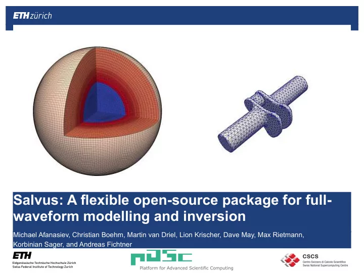
Salvus: A flexible open-source package for full- waveform modelling and inversion Michael Afanasiev, Christian Boehm, Martin van Driel, Lion Krischer, Dave May, Max Rietmann, Korbinian Sager, and Andreas Fichtner 1.12.2014

Full waveform inversion ∂ 2 t u ( x ) � r · σ ( x ) � F = 0 σ ( x ) = c ( x ) : r u ( x )

Full waveform inversion ∂ 2 t u ( x ) � r · σ ( x ) � F = 0 σ ( x ) = c ( x ) : r u ( x ) A problem of optimal control over c , constrained by the wave equation.

Motivation σ ( x ) = c ( x ) : r u ( x ) Takes on a very different character …

Motivation Acoustic and attenuative 2D/3D propagation through tissue Elastic regional scale with topography σ ( x ) = c ( x ) : r u ( x ) Takes on a very different character … Elastic/Acoustic/ 2D/3D, Elastic/Acoustic coupling, Gravity coupling, 3D, Topography, Attenuation attenuative

Motivation Acoustic and attenuative 2D/3D propagation through tissue Elastic regional scale with topography Elastic/Acoustic/ 2D/3D, Elastic/Acoustic coupling, Gravity coupling, 3D, Topography, Attenuation attenuative

Motivation Acoustic and attenuative 2D/3D propagation through tissue Elastic regional scale with topography Elastic/Acoustic/ 2D/3D, Elastic/Acoustic coupling, Gravity coupling, 3D, Topography, Attenuation attenuative

Requirements ▪ Flexible and modular design, with support for the concurrent simulation of multiple coupled PDEs — composability ▪ Scalable, dimension independent spatial and temporal discretization ▪ Simple integration with external optimization libraries ▪ Correct and consistent solutions ▪ Speed

Flexible and modular design, with support for the concurrent simulation of multiple coupled PDEs

Modular design Coupling physics … Additional physics … Physics 2 Physics … Physics 1 Hex Quad FEM Basis 2 FEM Basis 1 FEM Basis … Shape Mapping 1 Shape Mapping 2 Shape Mapping … .

Modular design (Composability) Shape::computeJacobian(); Shape::interpolateParameters(); … Element::computeSymmetricGradient(); Element::applyGradTestAndIntegrate(); … Physics::computeStrain(); Physics::computeStress(); … AdditionalPhysics::modifyStress(); … CouplingPhysics::computeCouplingTerm(); … … need to change any one of these independently.

Modular design: a solution with template mixins template <typename Element> MatrixXd Elastic2D<Element>::computeStiffnessTerm(const Eigen::MatrixXd &u) { // strain ux_x, ux_y, uy_x, uy_y. mStrain.leftCols<2>() = Element::computeGradient(u.col(0)); mStrain.rightCols<2>() = Element::computeGradient(u.col(1)); // compute stress from strain. mStress = computeStress(mStrain); // temporary matrix to hold directional stresses. Matrix<double,Dynamic,2> temp_stress(Element::NumIntPnt(), 2); // compute stiffness. temp_stress.col(0) = mStress.col(0); temp_stress.col(1) = mStress.col(2); mStiff.col(0) = Element::applyGradTestAndIntegrate(temp_stress); temp_stress.col(0) = mStress.col(2); temp_stress.col(1) = mStress.col(1); mStiff.col(1) = Element::applyGradTestAndIntegrate(temp_stress); return mStiff; }

Modular design: a solution with template mixins template <typename Element> MatrixXd Elastic2D<Element>::computeStiffnessTerm(const Eigen::MatrixXd &u) { // strain ux_x, ux_y, uy_x, uy_y. mStrain.leftCols<2>() = Element::computeGradient(u.col(0)); mStrain.rightCols<2>() = Element::computeGradient(u.col(1)); // compute stress from strain. mStress = computeStress(mStrain); // temporary matrix to hold directional stresses. Matrix<double,Dynamic,2> temp_stress(Element::NumIntPnt(), 2); // compute stiffness. temp_stress.col(0) = mStress.col(0); temp_stress.col(1) = mStress.col(2); mStiff.col(0) = Element::applyGradTestAndIntegrate(temp_stress); temp_stress.col(0) = mStress.col(2); temp_stress.col(1) = mStress.col(1); mStiff.col(1) = Element::applyGradTestAndIntegrate(temp_stress); return mStiff; }

Modular design: a solution with template mixins template <typename Physics> MatrixXd Attenuation<Physics>::computeStiffnessTerm(const Eigen::MatrixXd &u) { strain = Physics::computeGradient(u); /* Modify strain by subtracting from memory variable equations… */ stress = Physics::computeStress(strain); stiff = Physics::applyGradTestAndIntegrate(stress); return stiff; }

Modular design: a solution with template mixins Building up elements … QuadP1 QuadP2 TensorBasis Acoustic Elastic2D Elastic3D Cpl2Acoustic Cpl2Elastic Attenuation …

Modular design: a solution with template mixins Building up elements … Adding attenuation to surface elements … . QuadP1 QuadP2 ElementAdapter< TensorBasis Attenuation< Acoustic Elastic2D< Elastic2D Quad< Elastic3D QuadP2>>>> AtnElasticQuadP1; Cpl2Acoustic Cpl2Elastic Attenuation …

Modular design: a solution with template mixins Building up elements … Adding attenuation to surface elements … . QuadP1 QuadP2 ElementAdapter< TensorBasis Attenuation< Acoustic Elastic2D< Elastic2D Quad< Elastic3D QuadP2>>>> AtnElasticQuadP1; Cpl2Acoustic Cpl2Elastic Attenuation Adding coupling to CMB … . … ElementAdapter< CoupleToAcoustic< Elastic2D< Quad< QuadP1>>>> AtnElasticQuadP1;

Modular design: a solution with template mixins // Get values from distributed array. mesh->pullElementalFields(); // Compute element integrals. for (auto &elm: elements) { // Get relevant values. u = mesh->getFields(elm->closure()); // Compute stiffness. ku = elm->computeStiffnessTerm(u); All in one element loop … // Compute surface integral. s = elm->computeSurfaceIntegral(u); // Compute source term. f = elm->computeSourceTerm(time); // Compute acceleration. a = f - ku + s // Assemble. mesh->pushFields(elm->closure()); } // Push values to distributed array. mesh->pushElementalFields();

Flexible spatial and temporal discretization

Flexible spatial discretization: Builtin python- based meshing tools 2D applications Exploration scale (with topography) Planets (Mars, Europa, … )

Flexible spatial discretization: PETSc DMPLEX An example with coupling Red: fluid Blue: solid

Flexible spatial discretization: PETSc DMPLEX An example with coupling Red: fluid Blue: solid

Flexible spatial discretization: PETSc DMPLEX v1 e2 v3 e5 v5 e1 f1 e4 f2 e7 (fluid) (solid) f2 (solid) v2 (fluid) e3 v4 (solid) e6 v6 f1 (fluid)

Flexible spatial discretization: PETSc DMPLEX v1 e2 v3 e5 v5 v1 e2 v3 e5 v5 e1 f1 e4 f2 e7 e1 f1 e4 f2 e7 (fluid) (solid) f2 f2 (solid) v2 e3 v4 e6 v6 v2 e3 v4 e6 v6 v1 v2 v3 v4 v5 v6 f1 (fluid) f1 e1 e2 e3 e4 e5 e6 e7 f1 f2 (fluid) (solid)

Flexible spatial discretization: PETSc DMPLEX v1 e2 v3 e5 v5 v1 e2 v3 e5 v5 e1 f1 e4 f2 e7 e1 f1 e4 f2 e7 (fluid) (solid) f2 (solid) f2 v2 e3 v4 e6 v6 v2 e3 v4 e6 v6 v1 v2 v3 v4 v5 v6 f1 f1 (fluid) e1 e2 e3 e4 e5 e6 e7 f1 f2 (fluid) (solid) element_vector.push_back( ElasticCplAcousticQuadP1(options));

Integration with external optimization routines (salvus_opt)

Wavefield Compression Time-domain full-waveform inversion requires massive storage capabilities to store the forward wavefield. Goal: Find a good tradeoff between memory requirements and computational overhead by using customized compression methods. 27

Line-Search with Inexact Gradients inexact gradient minimum exact gradient (unknown) contour lines of misfit functional m k 28 |

Line-Search with Inexact Gradients inexact gradient minimum exact gradient (unknown) contour lines of misfit functional m k 29 |

Line-Search with Inexact Gradients inexact gradient minimum exact gradient (unknown) contour lines of misfit functional m k 30 |

Line-Search with Inexact Gradients inexact gradient minimum exact gradient (unknown) contour lines of misfit functional m k Compression thresholds can be chosen adaptively based on ➢ the norm of the inexact gradient, ➢ the ratio of actual and predicted misfit reduction. Convergence can be ensured if the relative error is smaller than 50%. 31 |

Wavefield Compression Substantial reduction of memory • Prediction-correction on ✦ requirements and I/O operations at hierarchical grids negligible extra costs. Requantization ✦ 200 TB per event • Re-interpolation with sliding- ✦ window cubic splines Using approximate gradients does not • significantly slow down the rate of convergence to solve the inverse problem. 4 = p 2 The error in the inexact gradients can be • = p controlled such that the lossy compression 1 = p does not significantly affect the inverted 0 = results. p 32