Rotations in the 2D Plane Trigonometric addition formulas: sin( + - - PDF document

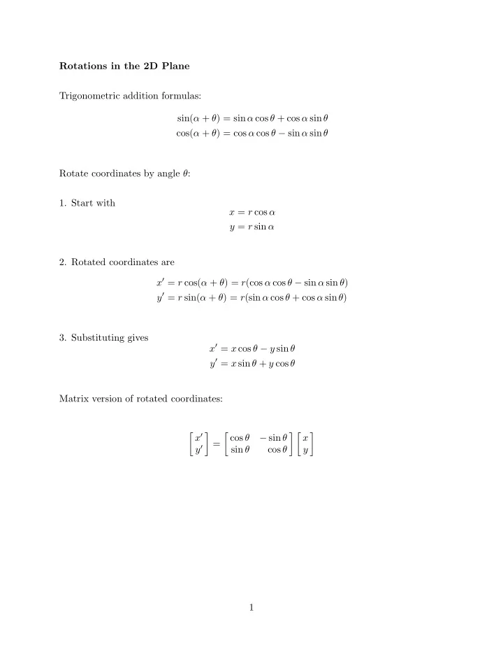
Rotations in the 2D Plane Trigonometric addition formulas: sin(α + θ) = sinα cos θ + cos α sinθ cos(α + θ) = cos α cos θ − sinα sinθ Rotate coordinates by angle θ:

• 1. Start with

x = r cos α y = r sin α

• 2. Rotated coordinates are

x′ = r cos(α + θ) = r(cos α cos θ − sin α sin θ) y′ = r sin(α + θ) = r(sin α cos θ + cos α sinθ)

• 3. Substituting gives

x′ = x cos θ − y sin θ y′ = x sin θ + y cos θ Matrix version of rotated coordinates:

• x′

y′

• =
• cos θ

− sin θ sin θ cos θ x y

• 1

Complex Numbers

• Both multiplication and addition are associative and commutative.
• If x = a + bi, define the conjugate of x, denoted ¯

x, to be a − bi.

• Define the norm of x, denoted ||x||, by

||x||2 = √ x¯ x =

• (a + bi) · (a − bi) =
• a2 + b2
• ||xy|| = ||x|| · ||y||
• Let x=a+bi, then

x · ¯ x ||x||2 = 1 and therefore x−1 = a a2 + b2 − b a2 + b2 i

• Complex numbers form a field. They also form a normed division algebra.
• Multiplication by a complex number with norm one is a rotation.

2

Rotations in 3D Space z-axis: Rz =   cos θ − sinθ sinθ cos θ 1   x-axis: Rx =   1 cos θ − sin θ sinθ cos θ   y-axis: Ry =   sin θ cos θ 1 cos θ − sinθ   3

Rotation about an Arbitrary Axis

• 1. Rotate around the z-axis until the arbitrary axis is in the zx-plane.
• 2. Rotate around the y-axis until the arbitrary axis coincides with the x-axis.
• 3. Rotate around the x-axis by angle θ.
• 4. Undo the rotations around the y-axis and z-axis.

A = RT

z RT y RxRyRz

If the unit vector (nx, ny, nz) is in the direction of the arbitrary axis, then rotation around this axis corresponds to multiplying by the following matrix where t = (1 − cos θ): A =   n2

xt + cos θ

nxnyt − nx sin θ nxnzt + ny sin θ nxnyt + nx sin θ n2

yt + cos θ

nynzt − nx sin θ nxnzt − ny sin θ nynzt + nx sin θ n2

zt + cos θ

  4

Some Linear Algebra

• Rotation is a linear transformation and therefore can be represented by a matrix.
• Rotation preserves distances and angles. Therefore, it preserves dot products.

Av · Aw = v · w

• If v =

  1   and w =   1  , then Av · Aw = a11a12 + a21a22 + a31a32 = 1 · 0 + 0 · 1 + 0 · 0 = 0

• All the columns of A are perpendicular to each other.
• Av · Av = a11a11 + a21a21 + a31a31 = 1. All columns have unit length.
• A is an orthonormal matrix.
• ATA = I
• (det A)2 = 1
• Since a rotation preserves handedness of the coordinate system, det A = 1
• A matrix is a rotation matrix if and only if it is orthonormal with determinant 1.

Proposition: Composition of two rotations is a rotation. Proof: Product of orthonormal matrices with determinant 1 is orthonormal with determi- nant 1. 5

Finding the Axis and Angle of a Rotation Matrix Axis: Since A is a rotation, we know that the matrix equation Ax = x has a solution. Solving gives (a23 − a32, a31 − a13, a12 − a21) Angle of rotation: tr(A) = tr((CRx)CT) = tr(CTCRx) = tr(Rx) = 1 + 2 cos θ θ = cos−1 tr(A) − 1 2

• .

6

Quaternion Histroy

Sir W illiam Row an Ham ilton

1805 - 1865 Lived in Dublin Discovered Quaternions on October 16, 1843

file:///C|/Documents%20and%20Settings/sjanke/Desktop/Quaternion/QHistory1.html10/11/2005 8:35:08 AM

Quaternion Histroy

Plaque on Brougham Bridge over the Royal Canal

Commemorating Hamilton's discovery of quaternions on October 16, 1843

file:///C|/Documents%20and%20Settings/sjanke/Desktop/Quaternion/QHistory2.html10/11/2005 8:35:22 AM

Quaternion Algebra:

• Take all objects of the form a + bi + cj + dk.
• Define ij = k,

jk = i, ki = j, i2 = −1, j2 = −1, k2 = −1

• Note ij = −ji,

jk = −kj, ik = −ki.

• Use the distributive property to multiply:

(a1 + b1i + c1j + d1k) × (a2 + b2i + c2j + d2k) =(a1a2 − b1b2 − c1c2 − d1d2) + (a1b2 + a2b1 + c1d2 − c2d1)i + (a1c2 + a2c1 + b2d1 − b1d2)j + (a1d2 + a2d1 + b1c2 − b2c1)k

• qr does not necessarily equal rq. Quaternion algebra is not commutative.

7

More Quaternion Algebra

• Define the conjugate of q by ¯

q = a − bi − cj − dk.

• Then q¯

q = a2 + b2 + c2 + d2 and define ||q|| = √q¯

• q. We have ||qp|| = ||q|| · ||p||.
• The quaternions form a skew field and is a normed division algebra.
• There is a natural correspondence between the number q = a + bi + cj + dk and the

vector (a, b, c, d).

• Think of a quaternion as a scalar plus a 3D vector:

q = a + bi + cj + dk = a + v = ||q||(cos α + sin α n)

• Think of a quaternion as a combination of complex numbers C1 = a1 + b1i and

C2 = a2 + b2i. q = C1 + C2j = a1 + b1i + a2j + b2k 8

Yet More Quaternion Algebra

• Take quaternions p = p0 +

p and q = q0 + q, then pq = (p0q0 − p · q) + p0 q + q0 p + p × q

• Take a quaternion q and a vector

v in R3. q v ¯ q = (q2

0 − |

q|2) v + 2q0( q × v) + 2( q · v) q

• Suppose

v = k q, then q v ¯ q = (q2

0 − |

q|2)k q + 2q0( q × k q) + 2( q · k q) q = (q2

0 − |

q|2)k q + 2( q · k q) q = q2

0k

q − k| q|2 q + 2k| q|2 q = k(q2

0 + |

q|2) q = k q

• Rotation: If q = cos θ

2 +sin θ 2

q, then q v ¯ q is the vector resulting from rotating v around axis q by angle θ.

• Multiplying two unit quaternions composes the two rotations:

q2 (q1 v ¯ q1) ¯ q2 = (q2 q1) v (¯ q1 ¯ q2) = q v ¯ q 9

Conversion of Quaternion to Matrix Start with a unit quaternion q = d + ai + bj + ck The the corresponding rotation matrix is:   1 − 2b2 − 2c2 2ab + 2dc 2ac − 2db 2ab − 2dc 1 − 2a2 − 2c2 2bc + 2da 2ac + 2db 2bc − 2da 1 − 2a2 − 2b2   10

Operation Counts Applying Matrix: 9 multiplications and 6 additions Applying Quaternion: 23 multiplications and 8 additions Compose Matrices: 27 multiplications and 18 additions Compose Quaternions: 12 multiplications and 32 additions Convert Quaternion to Matrix: 16 multiplications and 10 additions Storage: Matrix (9 floating point), Quaternion(4 floating point) 11

Calculating Quaternion Multiplication q1 = d1 + a1i + b1j + c1k q2 = d2 + a2i + b2j + c2k q = d + ai + bj + ck q = q1q2 A = (d1 + a1)(d2 + a2) B = (c1 − b1)(b2 − c2) C = (a1 − d1)(b2 − c2) D = (b1 + c1)(a2 − d2) E = (a1 + c1)(a2 + b2) F = (a1 − c1)(a2 − b2) G = (d1 + b1)(d2 − c2) H = (d1 − b1)(d2 + c2) d = B + (−E − F + G + H)/2 a = A − (E + F + G + H)/2 b = −C + (E − F + G − H)/2 c = −D + (E − F − G + H)/2 8 Multiplications 4 Divisions 32 Additions 12

Spherical Interpolation of Quaternions slerp(q1, q2, t) = sin((1 − t)φ) sin φ q1 + sin(αt) sinφ q2 13

Quaternion Histroy

History of Vector Analysis

• Hamilton discovers quaternions 1843
• Gauss may have discovered quaternions independently

somewhat earlier.

• Mobius: Barycentric coordinates
• Grassmann 1844
• Tait and Maxwell (1873 treatise using quaternions and

standard vectors)

• Gibbs and Heaviside 1880's
• Debate in Nature 1890's (Tait: "Don't spoon feed the

public.")

file:///C|/Documents%20and%20Settings/sjanke/Desktop/Quaternion/QHistory3.html10/11/2005 8:35:37 AM

The Normed Division Algebras

• R (real numbers) is a commutative associative normed division algebra (with trivial

conjugation).

• C (complex numbers) is a commutative associative normed division algebra with (non-

trivial conjugation).

• H (quaternions) is a associative normed division algebra (non-commutative).
• O (octonions) is a normed division algebra (non-associative and non-commutative).

Lemma: Z=Y+iY is a division algebra just when Y is an associative division algebra. 14