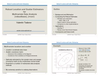
Robust scatter regularization G. Haesbroeck and C. Croux University - PowerPoint PPT Presentation

Robust scatter regularization G. Haesbroeck and C. Croux University of Li` ege - University of Leuven COMPSTAT 2010 G. Haesbroeck and C. Croux (Belgium) Robust scatter regularization COMPSTAT 2010 1 / 14

Introduction Let X = ( X 1 , . . . , X p ) T be a p -dimensional random vector with X i ∼ N p ( µ, Σ) where µ is the mean and Σ is the nonsingular covariance matrix. Aim: Estimate, in a robust way, µ and Θ = Σ − 1 (concentration matrix) using a sample of size n . G. Haesbroeck and C. Croux (Belgium) Robust scatter regularization COMPSTAT 2010 2 / 14

Maximum Likelihood estimator The ML estimator of ( µ, Θ) maximizes n � log(det(Θ)) − 1 ( x i − µ ) T Θ( x i − µ ) . n i =1 When the sample covariance matrix S is nonsingular, µ ML , ˆ x , S − 1 ) . (ˆ Θ ML ) = (¯ When S is singular (e.g. when n < p ), the ML estimator does not exist. G. Haesbroeck and C. Croux (Belgium) Robust scatter regularization COMPSTAT 2010 3 / 14

Regularized Maximum Likelihood estimator The Regularized ML estimator of ( µ, Θ) maximizes n � log(det(Θ)) − 1 ( x i − µ ) T Θ( x i − µ ) − λ J (Θ) , n i =1 where λ ≥ 0 is the penalty parameter and J is a penalty function. Typical choices: L 1 -norm: J (Θ) = � p i , j =1 | Θ ij | L 2 -norm: J (Θ) = � p i , j =1 Θ 2 ij ... G. Haesbroeck and C. Croux (Belgium) Robust scatter regularization COMPSTAT 2010 4 / 14

Breakdown Point Roughly speaking, the breakdown point is the smallest fraction of contamination that can drive the estimator over all bounds. For a scatter estimator, breakdown can occur due to explosion: λ 1 (Θ) → ∞ or implosion: λ p (Θ) → 0 with λ p (Θ) ≤ . . . ≤ λ 1 (Θ) . G. Haesbroeck and C. Croux (Belgium) Robust scatter regularization COMPSTAT 2010 5 / 14

Breakdown of the Regularized ML procedure µ = 0 , Σ = I p and x ′ n = x n + xe 1 0.4 0.3 λ p (Θ) 0.2 0.1 0.0 0 5 10 15 20 x G. Haesbroeck and C. Croux (Belgium) Robust scatter regularization COMPSTAT 2010 6 / 14

Breakdown of the Regularized ML procedure µ = 0 , Σ = I p and x ′ n = x n + xe 1 0.4 0.3 λ p (Θ) 0.2 0.1 0.0 0 5 10 15 20 x Robust alternatives are needed! G. Haesbroeck and C. Croux (Belgium) Robust scatter regularization COMPSTAT 2010 6 / 14

Minimum Covariance Determinant estimator Find a subsample H of size h (with n 2 ≤ h ≤ n ) minimizing the generalized variance log(det(Σ H )) (where Σ H is the covariance matrix based on the h points). The location and scatter MCD estimates are given by the mean and covariance matrix of the optimal subsample. G. Haesbroeck and C. Croux (Belgium) Robust scatter regularization COMPSTAT 2010 7 / 14

Regularized MCD estimator Find a subsample H of size h maximizing � log(det(Θ H )) − 1 ( x i − µ H ) T Θ H ( x i − µ H ) − λ J (Θ H ) h i ∈ H The regularized MCD estimator is given by the regularized ML estimator computed on the optimal subsample. G. Haesbroeck and C. Croux (Belgium) Robust scatter regularization COMPSTAT 2010 8 / 14

Properties of the Regularized MCD estimator A. Robustness The finite-sample breakdown point for joint location and scatter of the Regularized MCD estimator is equal to Σ MCD ); X ) = min( h , n − h + 1) µ MCD , ˆ ε ∗ ((ˆ n where n 2 ≤ h ≤ n is the number of observations selected in the MCD solution. µ MCD , ˆ In particular, for h = n / 2, ε ∗ ((ˆ Σ MCD ); X ) = 1 / 2 . G. Haesbroeck and C. Croux (Belgium) Robust scatter regularization COMPSTAT 2010 9 / 14

Properties of the Regularized MCD estimator B. Computation Iterative algorithm: µ 0 , ˆ µ k , ˆ µ k +1 , ˆ (ˆ Θ 0 ) → . . . → (ˆ Θ k ) → (ˆ Θ k +1 ) → . . . µ 0 , ˆ (ˆ Θ 0 ) : Regularized ML estimator based on a random subset of 2 observations iteration k to k + 1 by means of a C − step works for n < p G. Haesbroeck and C. Croux (Belgium) Robust scatter regularization COMPSTAT 2010 10 / 14

Simulations Clean setting: n = p = 50, Σ ii = 1 and Σ ij = 0 . 5 I ( i , j ≤ 9) for all i � = j . Contaminated setting: 5% of shift and correlation outliers (intermediate or extreme) L 1 penalty ML MCD KL( � KL( � MSE(ˆ µ ) Θ) MSE(ˆ µ ) Θ) Clean 0.98 6.94 1.43 6.46 5% Intermediate 1.70 9.76 1.42 6.53 5% Extreme 200.89 17.58 1.41 6.53 where KL ( � Θ) = − log(det( � Θ)) + tr( � ΘΣ) − ( − log(det(Σ − 1 )) + p ) G. Haesbroeck and C. Croux (Belgium) Robust scatter regularization COMPSTAT 2010 11 / 14

Applications Detection of outliers in high dimensional data (with n < p or n / p small). Robust graphical modelling Robust regularized regression G. Haesbroeck and C. Croux (Belgium) Robust scatter regularization COMPSTAT 2010 12 / 14

Detection of outliers n = p = 50, Σ ii = 1 and Σ ij = 0 . 5 I ( i , j ≤ 9) for all i � = j , 5% of shift and correlation outliers Regularized MCD robust distances 300 200 100 0 0 2 4 6 8 10 Regularized ML Mahalanobis distances G. Haesbroeck and C. Croux (Belgium) Robust scatter regularization COMPSTAT 2010 13 / 14

Conclusions Robust regularized scatter estimation is available. Other robust multivariate estimators can also be adapted to the penalized setting (e.g. M estimator,...). Still room for further research. G. Haesbroeck and C. Croux (Belgium) Robust scatter regularization COMPSTAT 2010 14 / 14