Robust and Efficient Methods of Inference for Non-Probability - PowerPoint PPT Presentation
Robust and Efficient Methods of Inference for Non-Probability Samples: Application to Naturalistic Driving Data Ali Rafei 1 , Michael R. Elliott 1 , Carol A.C. Flannagan 2 1 Michigan Program in Survey Methodology 2 University of Michigan
Robust and Efficient Methods of Inference for Non-Probability Samples: Application to Naturalistic Driving Data Ali Rafei 1 , Michael R. Elliott 1 , Carol A.C. Flannagan 2 1 Michigan Program in Survey Methodology 2 University of Michigan Transportation Research institute JPSM/MPSM Seminar 2020 September 30 Rafei, Ali (MPSM) Robust Inference for Non-Probability Samples JSM 2020 1 / 35
Problem statement Probability sampling is the gold standard for finite population inference. The 21 st century witnesses re-emerging non-probability sampling. The response rate is steadily declining. 1 Massive unstructured data are increasingly available. 2 Convenience samples are easier, cheaper and faster to collect. 3 Rare events, such as crashes, require long-term followup. 4 Rafei, Ali (MPSM) Robust Inference for Non-Probability Samples JSM 2020 2 / 35
Naturalistic Driving Studies (NDS) TRIP One real-world application of sensor-based Big Data. VEHICLE Driving behaviors are monitored via instrumented vehicles. NDS A rich resource for exploring crash causality, traffic safety, DRIVER and travel dynamics. EVENT Rafei, Ali (MPSM) Robust Inference for Non-Probability Samples JSM 2020 3 / 35
Strategic Highway Research Program 2 Launched in 2010, SHRP2 is the largest NDS conducted to date. Participants were ∼ 3,150 volunteers from six sites across the U.S. ∼ 5M trips & ∼ 50M driven miles were recorded. (Trip? time interval during which vehicle is on) Major challenges: SHRP2 is a non-probability sample. 1 Youngest/eldest groups were oversampled. 2 Only six sites have been studied. 3 Rafei, Ali (MPSM) Robust Inference for Non-Probability Samples JSM 2020 4 / 35
Strategic Highway Research Program 2 Launched in 2010, SHRP2 is the largest NDS conducted to date. Participants were ∼ 3,150 volunteers from six sites across the U.S. ∼ 5M trips & ∼ 50M driven miles were recorded. (Trip? time interval during which vehicle is on) Major challenges: SHRP2 is a non-probability sample. 1 Youngest/eldest groups were oversampled. 2 Only six sites have been studied. 3 Rafei, Ali (MPSM) Robust Inference for Non-Probability Samples JSM 2020 4 / 35
Strategic Highway Research Program 2 Launched in 2010, SHRP2 is the largest NDS conducted to date. Participants were ∼ 3,150 volunteers from six sites across the U.S. Participants' age group (yrs) ∼ 5M trips & ∼ 50M driven miles were recorded. 50 (Trip? time interval during which vehicle is on) 40 37.2 percent (%) Major challenges: 30 Study SHRP2 US Pop 20 19.3 18.4 18.1 SHRP2 is a non-probability sample. 17.1 1 14.1 13.8 11.5 10.6 10.9 10 9.3 7.6 7.4 Youngest/eldest groups were oversampled. 2 4.7 0 Only six sites have been studied. 15−24 25−34 35−44 45−54 55−64 65−74 75+ 3 Population size of resid. area (x1000) Rafei, Ali (MPSM) Robust Inference for Non-Probability Samples JSM 2020 4 / 35 50 43.1 42.6 40 33 percent (%) 30 Study 27.8 SHRP2 NHTS 20 14.3 10.6 9.8 10 9.1 5.3 4.2 0 <50 50−200 200−500 500−1000 1000+
Basic framework X 𝜌 Y Z Let’s define the following notations: B : Big non-probability sample 1 1 ? 1 R : Reference survey ? 2 . . X : Set of common auxiliary vars 3 . . . Y : Outcome var of interest 4 B . . Z : Indicator of being in B 5 . . . ? Considering MAR+positivity assumptions given X : 1 Quasi-randomization (QR): 0 1 ? Estimating pseudo-inclusion probabilities ( π B ) in B . ? R . ? Prediction modeling (PM): 2 0 Predicting the outcome var ( Y ) for units in R Combined sample Doubly robust Adjustment (DR): 3 Combining the two to further protect against model misspecification Rafei, Ali (MPSM) Robust Inference for Non-Probability Samples JSM 2020 5 / 35 Let combine B with R and define Z = I ( i ∈ B ) .
Basic framework X 𝜌 Y Z Let’s define the following notations: B : Big non-probability sample 1 1 1 R : Reference survey 2 . X : Set of common auxiliary vars 3 . . Y : Outcome var of interest 4 B . Z : Indicator of being in B 5 . . Considering MAR+positivity assumptions given X : 1 Quasi-randomization (QR): 0 1 ? Estimating pseudo-inclusion probabilities ( π B ) in B . ? R . ? Prediction modeling (PM): 2 0 Predicting the outcome var ( Y ) for units in R Combined sample Doubly robust Adjustment (DR): 3 Combining the two to further protect against model misspecification Rafei, Ali (MPSM) Robust Inference for Non-Probability Samples JSM 2020 5 / 35 Let combine B with R and define Z = I ( i ∈ B ) .
Basic framework X 𝜌 Y Z Let’s define the following notations: B : Big non-probability sample 1 1 ? 1 R : Reference survey 2 ? . X : Set of common auxiliary vars . 3 . . . Y : Outcome var of interest 4 B . . Z : Indicator of being in B 5 . . . Considering MAR+positivity assumptions given X : ? 1 Quasi-randomization (QR): 1 0 Estimating pseudo-inclusion probabilities ( π B ) in B . R . Prediction modeling (PM): 2 0 Predicting the outcome var ( Y ) for units in R Combined sample Doubly robust Adjustment (DR): 3 Combining the two to further protect against model misspecification Rafei, Ali (MPSM) Robust Inference for Non-Probability Samples JSM 2020 5 / 35 Let combine B with R and define Z = I ( i ∈ B ) .
Basic framework X 𝜌 Y Z Let’s define the following notations: B : Big non-probability sample 1 1 1 R : Reference survey 2 . X : Set of common auxiliary vars 3 . . Y : Outcome var of interest 4 B . Z : Indicator of being in B 5 . . Considering MAR+positivity assumptions given X : 1 Quasi-randomization (QR): 0 1 Estimating pseudo-inclusion probabilities ( π B ) in B . R . Prediction modeling (PM): 2 0 Predicting the outcome var ( Y ) for units in R Combined sample Doubly robust Adjustment (DR): 3 Combining the two to further protect against model misspecification Rafei, Ali (MPSM) Robust Inference for Non-Probability Samples JSM 2020 5 / 35 Let combine B with R and define Z = I ( i ∈ B ) .
Quasi-randomization Traditionally, propensity scores are used to estimate pseudo-weights (Lee 2006). PS weighting when R is epsem : n B y PW = 1 y i ∑ ¯ π B ( x i ) N i = 1 where under a logistic regression model, we have exp { x T i β } π B ( x i ) ∝ p i ( β ) = P ( Z i = 1 | x i ; β ) = i β } , ∀ i ∈ B 1 + exp { x T When R is NOT epsem , β can be estimated through a PMLE approach by solving: ∑ i ∈ B x i [ 1 − p i ( β )] − ∑ i ∈ R x i p i ( β ) / π R i = 0 (odds of PS) (Wang et al. 2020) 1 ∑ i ∈ B x i − ∑ i ∈ R x i p i ( β ) / π R i = 0 (Chen et al. 2019) 2 ∑ i ∈ B x i / p i ( β ) − ∑ i ∈ R x i / π R i = 0 (Kim 2020) 3 Rafei, Ali (MPSM) Robust Inference for Non-Probability Samples JSM 2020 6 / 35
Quasi-randomization Traditionally, propensity scores are used to estimate pseudo-weights (Lee 2006). PS weighting when R is epsem : n B y PW = 1 y i ∑ ¯ π B ( x i ) N i = 1 where under a logistic regression model, we have exp { x T i β } π B ( x i ) ∝ p i ( β ) = P ( Z i = 1 | x i ; β ) = i β } , ∀ i ∈ B 1 + exp { x T When R is NOT epsem , β can be estimated through a PMLE approach by solving: ∑ i ∈ B x i [ 1 − p i ( β )] − ∑ i ∈ R x i p i ( β ) / π R i = 0 (odds of PS) (Wang et al. 2020) 1 ∑ i ∈ B x i − ∑ i ∈ R x i p i ( β ) / π R i = 0 (Chen et al. 2019) 2 ∑ i ∈ B x i / p i ( β ) − ∑ i ∈ R x i / π R i = 0 (Kim 2020) 3 Rafei, Ali (MPSM) Robust Inference for Non-Probability Samples JSM 2020 6 / 35
Quasi-randomization However, the PMLE approach is limited to the parametric models. One may be interested in applying more flexible non-parametric methods. Denote δ i = δ B i + δ R i . With an additional assumption B ∩ R = ∅ , one can show π B i = P ( δ B i = 1 | x i , π R i ) = P ( δ i = 1 | x i , π R i ) P ( Z i = 1 | x i , π R i ) π R i = P ( δ R i = 1 | x i , π R i ) = P ( δ i = 1 | x i , π R i ) P ( Z i = 0 | x i , π R i ) Propensity Adjusted Probability weighting (PAPW): p i ( β ∗ ) π B i ( x ∗ i ; β ∗ ) = π R 1 − p i ( β ∗ ) , ∀ i ∈ B i i ] , and β ∗ can be estimated through the regular MLE. where x ∗ i = [ x i , π R This is especially advantageous when applying a broader range of predictive methods. Rafei, Ali (MPSM) Robust Inference for Non-Probability Samples JSM 2020 7 / 35
Quasi-randomization However, the PMLE approach is limited to the parametric models. One may be interested in applying more flexible non-parametric methods. Denote δ i = δ B i + δ R i . With an additional assumption B ∩ R = ∅ , one can show π B i = P ( δ B i = 1 | x i , π R i ) = P ( δ i = 1 | x i , π R i ) P ( Z i = 1 | x i , π R i ) π R i = P ( δ R i = 1 | x i , π R i ) = P ( δ i = 1 | x i , π R i ) P ( Z i = 0 | x i , π R i ) Propensity Adjusted Probability weighting (PAPW): p i ( β ∗ ) π B i ( x ∗ i ; β ∗ ) = π R 1 − p i ( β ∗ ) , ∀ i ∈ B i i ] , and β ∗ can be estimated through the regular MLE. where x ∗ i = [ x i , π R This is especially advantageous when applying a broader range of predictive methods. Rafei, Ali (MPSM) Robust Inference for Non-Probability Samples JSM 2020 7 / 35
Recommend
More recommend
Explore More Topics
Stay informed with curated content and fresh updates.
