Review & Finish CSPs Begin Logical Agents Constraint - PowerPoint PPT Presentation

Review & Finish CSPs Begin Logical Agents

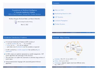
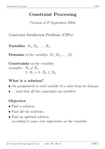
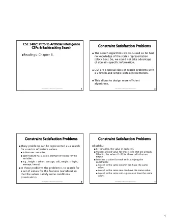
Constraint Satisfaction Problems Constraint Satisfaction Problems • What is a CSP? – Finite set of variables X 1 , X 2 , …, X n – Nonempty domain of possible values for each variable D 1 , D 2 , …, D n – Finite set of constraints C 1 , C 2 , …, C m Finite set of constraints C 1 , C 2 , …, C m • Each constraint C i limits the values that variables can take, • e.g., X 1 ≠ X 2 – Each constraint C i is a pair <scope, relation> • Scope = Tuple of variables that participate in the constraint. • Relation = List of allowed combinations of variable values. May be an explicit list of allowed combinations. May be an abstract relation allowing membership testing and M b b t t l ti ll i b hi t ti d listing. • CSP benefits – Standard representation pattern Standard representation pattern – Generic goal and successor functions – Generic heuristics (no domain specific expertise).

CSPs --- what is a solution? CSPs what is a solution? • A state is an assignment of values to some or all variables. A t t i i t f l t ll i bl – An assignment is complete when every variable has a value. – An assignment is partial when some variables have no values. • Consistent assignment – assignment does not violate the constraints • A solution to a CSP is a complete and consistent assignment. • Some CSPs require a solution that maximizes an objective function .

CSP as a standard search problem • A CSP can easily be expressed as a standard search problem. • Incremental formulation – Initial State : the empty assignment {} – Actions (3 rd ed.), Successor function (2 nd ed.) : Assign a value to an unassigned variable provided that it does not violate a constraint – Goal test : the current assignment is complete (by construction it is consistent) – Path cost : constant cost for every step (not really relevant) • C Can also use complete-state formulation f – Local search techniques (Chapter 4) tend to work well

Improving CSP efficiency Improving CSP efficiency • Previous improvements on uninformed search  introduce heuristics • For CSPS, general-purpose methods can give large gains in speed, e.g., – Which variable should be assigned next? – In what order should its values be tried? – Can we detect inevitable failure early? – Can we take advantage of problem structure? Note: CSPs are somewhat generic in their formulation, and so the heuristics are more general compared to methods in Chapter 4

Backtracking search Backtracking search function BACKTRACKING-SEARCH( csp ) return a solution or failure return RECURSIVE-BACKTRACKING( {} , csp ) function RECURSIVE-BACKTRACKING( assignment, csp ) return a solution or failure if assignment is complete then return assignment var  SELECT-UNASSIGNED-VARIABLE(VARIABLES[ csp ], assignment , csp ) for each value in ORDER-DOMAIN-VALUES( var, assignment, csp ) do if value is consistent with assignment according to CONSTRAINTS[ csp ] then add {var=value} to assignment result  RRECURSIVE-BACTRACKING( assignment, csp ) ( g , p ) if result  failure then return result remove {var=value} from assignment return failure

Minimum remaining values (MRV) (MRV) var  SELECT-UNASSIGNED-VARIABLE(VARIABLES[ csp ] assignment csp ) var  SELECT UNASSIGNED VARIABLE(VARIABLES[ csp ], assignment , csp ) • A.k.a. most constrained variable heuristic • Heuristic Rule : choose variable with the fewest legal moves – e.g., will immediately detect failure if X has no legal values

Degree heuristic for the initial variable variable • Heuristic Rule : select variable that is involved in the largest number of constraints on other unassigned variables. • Degree heuristic can be useful as a tie breaker. • In what order should a variable’s values be tried?

Least constraining value for value ordering value-ordering • • Least constraining value heuristic Least constraining value heuristic • Heuristic Rule: given a variable choose the least constraining value – leaves the maximum flexibility for subsequent variable assignments

Forward checking • Assign {Q=green} Assign {Q green} • Effects on other variables connected by constraints with WA – NT can no longer be green – NSW can no longer be green NSW can no longer be green – SA can no longer be green • MRV heuristic would automatically select NT or SA next

Forward checking • If V is assigned blue If V is assigned blue • Effects on other variables connected by constraints with WA – NSW can no longer be blue – SA is empty SA is empty • FC has detected that partial assignment is inconsistent with the constraints and backtracking can occur.

Arc consistency An Arc X  Y is consistent if • for every value x of X there is some value y consistent with x for every value x of X there is some value y consistent with x (note that this is a directed property) • Consider state of search after WA and Q are assigned: SA  NSW is consistent if SA bl SA=blue and NSW=red d NSW d

Arc consistency X  Y is consistent if • for every value x of X there is some value y consistent with x for every value x of X there is some value y consistent with x NSW  SA is consistent if • NSW=red and SA=blue NSW=blue and SA=???

Arc consistency • Can enforce arc-consistency: Can enforce arc consistency: Arc can be made consistent by removing blue from NSW • Continue to propagate constraints…. – Check V  NSW – Not consistent for V = red – Remove red from V f

Arc consistency • Continue to propagate constraints Continue to propagate constraints…. SA  NT is not consistent • – and cannot be made consistent and cannot be made consistent • Arc consistency detects failure earlier than FC

Arc consistency algorithm (AC-3) Arc consistency algorithm (AC 3) function AC-3( csp ) return the CSP, possibly with reduced domains inputs : csp , a binary csp with variables {X 1 , X 2 , …, X n } local variables: queue a queue of arcs initially the arcs in csp local variables: queue, a queue of arcs initially the arcs in csp while queue is not empty do ( X i , X j )  REMOVE-FIRST( queue ) if REMOVE-INCONSISTENT-VALUES( X i , X j ) then j for each X k in NEIGHBORS[ X i ] do add ( X i , X j ) to queue function REMOVE-INCONSISTENT-VALUES( X i , X j ) return true iff we remove a value removed  false removed  false for each x in DOMAIN[ X i ] do if no value y in DOMAIN[ X j ] allows (x,y) to satisfy the constraints between X i and X j then delete x from DOMAIN[ X i ]; removed  true return removed (from Mackworth, 1977)

K consistency K-consistency • Arc consistency does not detect all inconsistencies: – P Partial assignment {WA=red, NSW=red} is inconsistent. ti l i t {WA d NSW d} i i i t t • Stronger forms of propagation can be defined using the notion of k-consistency. • A CSP is k-consistent if for any set of k-1 variables and for any consistent assignment to those variables, a consistent value can always be assigned to any kth variable. – E.g. 1-consistency = node-consistency – E g 2 consistency E.g. 2-consistency = arc-consistency arc consistency – E.g. 3-consistency = path-consistency • Strongly k-consistent: – k consistent for all values {k k 1 k-consistent for all values {k, k-1, …2, 1} 2 1}

Local search for CSP Local search for CSP function MIN-CONFLICTS( csp, max_steps ) return solution or failure inputs : csp , a constraint satisfaction problem t i t ti f ti bl i t max_steps , the number of steps allowed before giving up current  an initial complete assignment for csp for i = 1 to max_steps do if current is a solution for csp then return current var  a randomly chosen, conflicted variable from VARIABLES[ csp ] value  the value v for var that minimize CONFLICTS( var,v,current,csp ) set var = value in current return failure

Graph structure and problem complexity • Solving disconnected subproblems – Suppose each subproblem has c variables out of a total of n . – Worst case solution cost is O(n/c d c ) , i.e. linear in n • Instead of O(d n ), exponential in n • E.g. n= 80, c= 20, d=2 E.g. n 80, c 20, d 2 2 80 = 4 billion years at 1 million nodes/sec. – – 4 * 2 20 = .4 second at 1 million nodes/sec

Tree-structured CSPs • • Theorem: Theorem: – if a constraint graph has no loops then the CSP can be solved in O(nd 2 ) time – linear in the number of variables! • Compare difference with general CSP, where worst case is O(d n )

Algorithm for Solving Tree- structured CSPs structured CSPs – Choose some variable as root, order variables from root to leaves such that every node’s parent precedes it in the ordering. • Label variables from X 1 to X n ) n ) 1 • Every variable now has 1 parent – Backward Pass • For j from n down to 2, apply arc consistency to arc [Parent( X j ), X j ) ] • Remove values from Parent( X j ) if needed – Forward Pass • For j from 1 to n assign X j consistently with Parent( X j )

Tree CSP Example Tree CSP Example G B

Tree CSP Example Tree CSP Example B Backw ard Pass B B R ( constraint R R G B G G propagation) G

Tree CSP Example Tree CSP Example B Backw ard Pass B B R ( constraint R R G B G G propagation) G Forw ard Pass B G R R G B ( assignm ent)