Rendering: Path Tracing II Adam Celarek Research Unit of Computer - PDF document
Rendering: Path Tracing II Adam Celarek Research Unit of Computer Graphics Instjtute of Visual Computjng & Human-Centered Technology TU Wien, Austria Path Tracing Basics (Last tjme) Materials / BSDF Path Tracing Algorithm
Rendering: Path Tracing II Adam Celarek Research Unit of Computer Graphics Instjtute of Visual Computjng & Human-Centered Technology TU Wien, Austria
Path Tracing Basics (Last tjme) Materials / BSDF Path Tracing Algorithm Next Event Estjmatjon (NEE) Russian Rouletue Details & Advanced (Now) Filtering Parallelisatjon Measuring Error Post-processing Path Tracing II (Adam Celarek) 2
Filtering Mission: Prevent sampling artefacts (aliasing) Path Tracing II (Adam Celarek) 3 source: own work Let’s start with filtering, the goal of which is to reduce or prevent sampling artefacts, or in other words aliasing. --- By the way, that picture is from Finland, the home of some very good computer graphics people..
Filtering With fjltering Without fjltering Path Tracing II (Adam Celarek) 4 source: Table scene designed by Olesya Jakob rendered with Nori We begin with an example.. On the left filtering was used, on the right not. The left looks a bit better when you compare **point** and **point**, but we can zoom in to see the difference more clearly..
Filtering With fjltering Without fjltering Path Tracing II (Adam Celarek) 5 source: Table scene designed by Olesya Jakob rendered with Nori There are these bright pixels **point** in high frequency areas, that clearly go away when we filter.. We have to look into it :)
Filtering We are in the main rendering loop, where we loop over pixels and the number of samples N, create a camera ray and then start tracing it. Path Tracing II (Adam Celarek) 6 Let me give some context about where filtering happens.. --- It is applied in the image coordinate system, where we see the pixels. That means that it lives in the main rendering loop, where we walk over pixels – in contrast to where we lived in the first part of the path tracing lecture, the recursive part.
Filtering We are in the main rendering loop, where we loop over pixels and the number of samples N, create a camera ray and then start tracing it. N samples Currently, you are using the box fjlter But let‘s go a step back for now and Current use only one sampling positjon pixel All N samples go through the centre Current pixel Path Tracing II (Adam Celarek) 7 In case you are taking the course at TU Wien, you implemented the box filter for assignment 2. That is, you chose random samples inside each pixel, and computed the average as an estimate of the pixel colour. That is already filtering. --- But, in order to make the explanation simpler, let’s go a step back for now and use only a sampling position in the pixel centre. In fact, this will be probably the way we will teach Monte Carlo next year.
Filtering Forget one screen dimension (works the same for higher dimensions) Path Tracing II (Adam Celarek) 8 Next, we’ll forget about one of the screen dimensions and start to think about a 1d function f(x). This is to make the explanation easier. All of the results also apply to the 2d screen we have in rendering. --- The green wavy line *point here and here*, is now the function that we want to sample and reconstruct as pixels on the screen. --- Here **point** you see the path integral formulation of light transport, because it’s shorter. --- It’s the integral *point f* of the light transport function *point fj* over all transport paths. You already learned in the first part of this lecture how to estimate the result using Monte Carlo. It’s the same process no matter the notation. --- But we can also use the recursive formulation. In that case, we would say that we have a function f that eats screen coordinates. The definition of the function tells to shoot a ray through that position, and compute the light recursively. That recursive computation returns the brightness at that position of the screen. --- For now we assume that f(x) is a continuous function – as opposed to a stochastic variable like in Monte Carlo Integration. That means that it always returns the same value for a given position, and positions are not discrete like monitor pixels.
Filtering Forget one screen dimension (works the same for higher dimensions) This is a sampling problem, much like with an analogue audio signal. We want to reconstruct the original signal afuer sampling Sample positjons Path Tracing II (Adam Celarek) 9 Now – we have that function *point f*, but only discrete pixels *point*, where each of them can display a single value. --- This is a sampling problem, very much like when you have to convert an analogue audio signal to a digital signal, and then play it. --- Let’s say, we go the simple and naive way and sample the signal at the centres of the pixels..
Filtering Sample positjons This is OK. The reconstructjon is Here not so much! faithful! Path Tracing II (Adam Celarek) 10 After sampling we have to reconstruct the signal, that is, draw it on the screen. As said, every pixel can have only one value, hence the boxy **point** reconstruction. --- This gives us a faithful representation of f if the frequency is low **point** on the left. By faithful I mean here, that the pixel values are close to the signal f, and that they would not change much if we shift the sample positions by a tiny bit (less than a pixel). --- So sampling the pixel centres works if the signal f has a low frequency, but it breaks down when the frequency becomes too large. The problem is called aliasing, you probably already heard about it. It happens when the sampling frequency is below the Nyquist frequency, which is 2x the signal frequency. --- There are 2 solutions: increase the sampling frequency or smooth the signal. We can’t really do the first, because it would change the rendering resolution, besides, when would we stop? But we can smooth the signal...
Filtering Solutjon: Smooth the signal before sampling with a low pass fjlter h(x) Sample positjons Path Tracing II (Adam Celarek) 11 Smoothing the signals means to apply a low pass filter h. We are filtering out high frequencies – hence the name of this section. --- Look at that, if we sample the signal f*h **point** at the centres of the pixels, it will give us faithful values to be used for the reconstruction as a pixel signal. --- You might think that we loose data, but that is not really the case as we couldn’t reproduce it anyway. --- Let’s look now into choices for the filter (or convolution) kernel h
Filtering What are the choices for smoothing kernel h(x)? Well, fjrst, what propertjes do we need? It should integrate to 1, otherwise the result would be brighter or darker than it should be. Well, actually, that is only needed theoretjcally, because our implementatjon will use normalisatjon anyways. The smoothing should be the right size Too small and too many of the large frequencies are retained Too large and we get visible blurring A shape that reduces artefacts (will not go into detail, see reading material). Path Tracing II (Adam Celarek) 12 But first, let’s look at the properties that we need. --- First, it should integrate to 1. This is because f(x) convoluted with h(x) should not be brighter or darker than the original signal f. This is more of a theoretical constrain, as any convolution kernel can be scaled and in fact we do that as part of the equation that we use. --- Obviously the kernel shouldn’t be too small or too large. In the first case we wouldn’t fix the reconstruction problem, or in the second case we would loose too much details. --- And finally, we need a good shape. Depending on the shape, some artefacts might appear. Different shapes can create different artefacts, and it’s generally a trade-off between these artefacts. But we won’t go into much detail there, because we would need much more sampling and reconstruction theory including the Fourier transform (not going there, not this time :)
Filtering What are the choices for smoothing kernel h(x)? box tent Gaussian (with cut-ofg) 1D 2D Path Tracing II (Adam Celarek) 13 Here we see some choices for the kernel. --- The first row is the 1d case and the cross section through the centre of the 2d case at the same time. --- The simplest is the box filter, which is super simple to implement. You just take the average of all pixel samples (we’ll talk more about how to implement later). It is common in super simple renderers, in case the author is too lazy to implement something better. It allows high-frequency sample data to leak into the reconstruction (PBR 7.8.1). --- The tent filter is slightly better --- And the Gaussian filter is reasonably good, but smooths the result. Did you see that it is clamped **point**. This is to limit it’s support.
Filtering What are the choices for smoothing kernel h(x)? Mitchell-Netravali-Filter with parameters (⅓, ⅓) source: Vierge Marie, Wikipedia Path Tracing II (Adam Celarek) (public domain) 14 There is a family of filters called Mitchell-Netravali. You can see that they can be negative **point**. This sharpens the result somewhat, but can cause an artefact caused ringing (depending on the parameters). --- The Mitchell-Netravali filter is considered the best by some, and I think it is a bonus task in assignment 3. --- Anyway, we will not go into further details in the differences. In my opinion, they are minute between Gaussian and Mitchell- Netravali.
Recommend
More recommend
Explore More Topics
Stay informed with curated content and fresh updates.
