Relativistic causality and no-signaling Pawe Horodecki Faculty of - - PowerPoint PPT Presentation

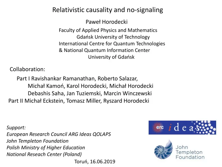
Relativistic causality and no-signaling

Faculty of Applied Physics and Mathematics Gdańsk University of Technology International Centre for Quantum Technologies & National Quantum Information Center University of Gdańsk Toruń, 16.06.2019 Support: European Research Council ARG Ideas QOLAPS John Templeton Foundation Polish Ministry of Higher Education National Reseach Center (Poland)

Paweł Horodecki Part I Ravishankar Ramanathan, Roberto Salazar, Michał Kamoń, Karol Horodecki, Michał Horodecki Debashis Saha, Jan Tuziemski, Marcin Winczewski Part II Michał Eckstein, Tomasz Miller, Ryszard Horodecki Collaboration:

• P. H., R. Ramanathan Nat. Comm. 10, 1701 (2019)
• R. Salazar, M. Kamon, D. Goyeneche, K. Horodecki, D. Saha, R. Ramanathan,
• P. H., arxiv:1712.01030
• M. Eckstein, P. H. , R. Horodecki and T. Miller, ,,Operational causality in space

time” arXiv:1902.05002

Mainly referred to:

Plan

PART I

• 1. Bell inequalities.
• 2. No-signaling boxes – beyond quantum mechanics
• 3. Digression: v-causal models

4 Can we go beyond no-signaling ? Relativistic causality 5.Relativistically causal boxes.

• 6. Surprising properties.

PART II

• 7. Causality of propagating potential statistics – concepts
• 8. Causality of propagating potential statistics – strong

restriction for propagation.

Quantum Physics and Quantum Entanglement

The breaktrough discovery of John Bell (1969)

John Bell (1928-1990)

A,A’,B,B’ =  1  A( B + B’) + A’ (B - B’) = AB + AB’ + A’B – A’B’  2 Assumption the both photons should simultanously carry its preexisting properties A, A’ (B,B’) equal either ,,I will pass = +1” or ,, I will not pass = - 1” (with respect to each of the two settings of the polariser).

  2 1 2 1 +   = 

Alice Bob

S

A=+1 A’=-1

B=-1 B’=-1

The Bell inequality in Clauser-Horne-Shimony-Holt (CHSH) variant

[J. F. Clauser, M. A. Horne, A. Shimony, A., R. A. Holt, PRL (1969)]

The breakthrough discovery of John Bell (1969)

• EPR idea in terms of local hidden variable

model (LHV) is refuted on quantum mechanical ground since the Bell inequality is violated

John Bell (1928-1990)

1 1

  2 1 2 1 +   = 

Alice Bob

S Settings choosen independently and randomly

BQ = A0 B0 + A0 B1 + A1 B0 - A1 B1| = 22 > 2 = BLHV

Bell experiment conditions

I. Space-like separation during the whole experiment

• III. ,,Free will” assumption

– local sources of random bits.

A B

• II. High enough efficiency detectors

(Bell inequality specific - 83% for CHSH). R Each of them correlated only with its future

(remember – correlations are reflexive: A is correlated with B  B is correlated with A !)

1

1

1 1

Bell inequalities - experiments

• I. Space-like separation

 (2013) during the whole experiment

• III. ,,Free will” assumption

– local sources of random bits.

• II. High enough efficiency detectors

(Bell inequality specific).  (2015)

Bell inequalities - experiments

• I. Space-like separation

 (2013) during the whole experiment

• III. ,,Free will” assumption

– local sources of random bits.

• II. High enough efficiency detectors

(Bell inequality specific).  (2015)

Bell inequalities - experiments

• I. Space-like separation

 (2013) during the whole experiment

• III. ,,Free will” assumption

– local sources of random bits.

• II. High enough efficiency detectors

(Bell inequality specific).  (2015)

Bell inequalities - experiments

• I. Space-like separation

 (2013) during the whole experiment

• III. ,,Free will” assumption

– local sources of random bits.

• II. High enough efficiency detectors

(Bell inequality specific).  (2015)

Bell Bell inequalities - experiments

• I. Space-like separation

 (2013) during the whole experiment

• III. ,,Free will” assumption

– local sources of random bits.

• II. High enough efficiency detectors

(Bell inequality specific).  (2015)

Bell experiment conditions

• I. Space-like separation

 (2013) during the whole experiment

• III. ,,Free will” assumption

– local sources of random bits

• II. High enough efficency detectors

(Bell inequality specific).

perfectly ,,unpredictible” coin

 (2015)

?

• Is he/she free (i) to make one experiment rather than another ?

(ii) to make it one way rather then another ?

Randomness and the freedom of an experimentalist

Obvious remark: free will is not equivalent to randomness at all

Technically speaking ,,ontic” randomness = fundamental nonpredictability is needed to perform the Bell test correctly …

R 1 1

perfectly ,,unpredictible” coin

Quantum information applications

Quantum Bell value and quantum security Purity of |  gives monogamy of quantum correlations: A max. entangled with B  not correlated with any E

A B E

  2 1 2 1 +   = 

Quantum   Violation of Bell inequality:

• Strong monogamy witness:

(BAB ) 2 + (BAE) 2  (22)2

[Toner, Verstraete (2006)]

• Strong certificate of maximal entanglement

(physical specification of the experiment devices *not* needed)

S

Device independent quantum security

x = 0 x = 1 y=0 y = 1 b =

1 1 1 1

a =

1 1 1 1

Cryptographic key: random, perfectly correlated, not known to anybody else.

  2 1 2 1 +   = 

Bell inequality violation guarantees device independent:

• Quantum cryptography [Vidick, & Vaziriani PRL (2012), inspired by Ekert PRL (1991)]
• Q. randomness expansion [Pironio et al. Nature (2009)], [Miller & Shi, J. of ACM (2016)]
• Q. randomness amplification see [ Chung, Shi & Wu, arXiv:1402.4797 ,

, review Acin & Massanes, Nature (2016)]).

• Quntum communication complexity reduction

[Brukner, Zukowski, Pan & Zeilinger PRL (2004)], [Brassard et al. PRL (2006)], [Buhrman et al. PNAS (2016)]

Other applications include:

Beyond quantum ?

So far we assumed (i) quantum mechanics + (ii) Bell inequality violation (experimental assumptions)

However the inequality violation guarantees much more: the ,,ontic” lack of preexistence of the properties before the measurements independently on the underlying physics (quantum or not).

Is there any chance to exploit that ? pLHV(AB|xy) =  p(A|x) p (B|y) p() d

Bell inequality-based quantum cryptography secure against ,,post-quantum” attack ,,Focus: Thwarting Post-Quantum Spies”

June 30, 2005• Phys. Rev. Focus 15, 2

“Uncrackable” quantum cryptography can thwart spies even if today’s quantum theory is replaced by something better–as long as it remains impossible to send messages faster than light.

[ J. Barrett, L. Hardy, A. Kent, Phys. Rev. Lett. (2005) ]

Bell inequality-based quantum cryptography secure against ,,post-quantum” attack

[ J. Barrett, L. Hardy, A. Kent, Phys. Rev. Lett. (2005) ]

Assumptions leading to the success: 1) Specific Bell inequality violation (chain inequality) 2) No-signaling condition for space-like separated labs:

x = 0 x = 1 y=0 y = 1 b

a

(post)-quantumly correlated state Independent statistics – to avoid faster-than-light telegraph

Quantum mechanics not assumed, only its ,,phenomenology”

• ie. correlations leading to violation of some Bell inequality.

Motivation for studying NS

1) Put ultimate limits for information processing in *any* future physical theory. 2) Look at quantum mechanics ,,from outside”. (what can be reproduced without referring to the algebraic structure) Foundations of physics perspective: Find (possibly ) new protocols in quantum information processing (sometimes reduction of mathematical formalism may help). Practical perspective:

Theory of ,,no-signaling boxes”

x = 0 x = 1 y=0 y = 1 b

a

[S. Popescu, D. Rohlich, Found. Phys. 24, 379 (1994)]

{ p(ab|xy) }

x y

a b ,,Boxes”: statistics of some measurements No-signaling conditions: ap(ab|xy):=p(b|xy)= p(b|y) NS from the right to the left (plus the same for a →b, x → y, ‚‚right” ‚‚left” )

No-signaling condition for more parties (natural generalisation) Three parties: (i) ap(abc|xyz):=p(bc|xyz)= p(bc|yz) (ii) abp(abc|xyz):=p(c|xyz)= p(c|z) + the same for all permutations of subsystems Note that from (i) + (ii) the left-right no-signaling

• f bipartite box { p(bc|yz)} follows automatically.

{ p(abc|xyz) }

x z

a c

y

b

Subset of quantum statistics: example

1 1 1 1 1 1 1 1 S

a b

x=0 x=1 y=1 y=0 { p(ab|xy) }

Measurements statistics

Ax By|= ab=1 ab p(ab|xy) B B = A0 B0| +A0 B1|+ A1 B0| - A1 B1|= 22

  2 1 2 1 +   = 

Theory of ,,no-signaling boxes”

Difficuilty: quantum statistics never extremal

• usually some purely deterministic component.

Bell-CHSH experiment :

2 22

4

  2 1 2 1 +   = 

Quantum statistics Extremal no-signalling statistics Locally realistic statistics

*

!

1 1 1 1 1 1

a b

x y 1 1 1 1 1 1

a b

x y

1/2 1/2 1/2 1/2 1/2 1/2 1/2 1/2

1 1 1 1

Statistics from |

Theory of ,,no-signaling boxes”

Difficulty : quantum statistics is never extremal

• usually has some purely deterministc component

Classical

Q

No-signaling

Proof in [R. Ramanathan, J. Tuziemski, M. Horodecki, P. H. Phys. Rev. Lett. (2016)]

Quantum statistics

Bell- CHSH experiment:

Extremal no-signalling statistics Locally realistic statistics

*

  2 1 2 1 +   = 

Quantum statistics is not pure if seen from

• utside  naive purity-monogamy-based

approach to cryptography does not work.

( Berrett, Hardy & Kent used additional property of chain Bell inequality)

NC vs QM comparison (I) Monogamy relations exist

There are monogamy relations for Bell correlations ([Masanes, Acin, Gisin PRL (2006)],[Toner Proc. R. Soc. A (2009)], universal [Brukner, Pawlowski PRL (2009)] no of Bob labs = no of Bob’s settings)

Example: stronger monogamy for Bell function depending

• n XOR of ourcomes (a  b) :
• Take Bell inequality

B 

AB  RLHV(B) < RNS(B)

• Find how many settings C you need to remove at Bob site to

trivialise the inequality to B 

AB  RLHV(B) = RNS(B)

• The inequality must satisfy the monogamy relation

with C+1 Bob’s labs

i=1

C+1 B

𝐵𝐶𝑗  (C+1)RLHV(B)

Broken chain and monogamy

x1 x2 xN-1 xN y1 y2 yN-1 yN

…

correlations (solid) anticorrrelations (dashed)

BAB  RLHV(B) < RNS(B) = 1 B’AB  RLHV(B’) = RNS(B’) = 1 – 1/2N

Taking one setting out makes inequality trivial (classical = NS)

[R. Ramanathan, P.H. PRL (2014)]

B (chain, N)

AB + B (chain, N) AC  2 RLHV(B(chain, N))

graph

NC vs QM comparison (II) Purification usually does not exists but complete extension does

In QM any mixed state A can (i) be extended to a pure state  AB = | AB   AB| (purification) (ii) s. t. all its ansambles of A can be represented by measurements on B (complete extension) In NC all the above is true except of the purity of extension.

[M. Winczewski, T. Das, K. Horodecki, P. Horodecki, Ł. Pankowski, M. Piani, R. Ramanathan, No purification in all discrete theories and the power of the complete extension, arXiv:1810.02222]

NC vs QM (III) Purity = complete statistical independence with ,,environment”

In NC, like in quantum mechanics, if the box is pure (has no nontrivial convex decomposition) then any extension is trivial (product with environment).

  2 1 2 1 +   = 

Quantum statistics Extremal no-signalling statistics PERFECTLY CRYPTOGRAPHICALLY SECURE in ,,NS world” Locally realistic statistics

*

NS vs QM (IV) Some variants of security agains NS eavesdropper are possible

Example.- Partial solution to free-will problem. Randomness amplification against NS eavesdropper.

• R. Renner, R. Colbeck, Nat. Phys. (2012),
• R. Gallego, L. Masanes, De La Torre, C. Dhara, L. Aolita, A. AcínNat Comm. (2013)
• F. G.S.L. Brandão, R. Ramanathan, A. Grudka, K. Horodecki,
• M. Horodecki, P. H. , T. Szarek, H. Wojewódka, Nat. Comm. (2016)
• F. G.S.L. Brandão, K. Horodecki, M. Horodecki,
• P. H. , H. Wojewódka, Phys. Rev. Lett. (2016)
• H. Wojewodka, F. G. S. L. Brandao, A. Grudka, M. Horodecki, K. Horodecki, P. Horodecki,
• M. Pawlowski, R. Ramanathan, M. Stankiewicz, IEEE TIT (2017)
• R. Ramanathan, M. Horodecki, S. Pironio, K. Horodecki, P. H.,

Generic randomness amplification schemes using Hardy paradoxes arXiv:1810.11648

• III. ,,Free will” assumption

– local sources of random bits

(Need of perfectly unpredictible coin dismissed)

Understand/reproduce quantum mechanics from basic principles

LHV – Classical (LHV) Quantum (Q) No-signaling (NS)

Two approaches:

• A. Full derivation of Q from LIST of axioms
• L. Hardy, quant-ph/0101012 (2001),
• G. Chiribella, G. M. D'Ariano, P. Perinotti,

PRA (2010, 2011), arXiv:1506.00398 (2015)

• B. The best outer approximation of Q by a SINGLE

information-type (physically motivated) principle:

• No-signaling - Rohlich & Popescu PRA 94)
• No trivial communication complexity - Brassard et al. PRL (2006)
• Macroscopic locality - M. Navascues, H. Wunderlich P. R. Soc. (2009)
• Information casuality - Pawlowski et al. Nature (2009).
• Local orthogonality – T. Fritz et al. Nat. Comm. (2013)
• Almost quantum - M. Navascues et al., Nat. Comm. (2014)
• Remark. Second (B) more focused on future physical theories, but the first (A) – harder -

also may work in that way (as contains some qualitative principles itself).

Understand/reproduce quantum mechanics from basic principles

LHV – Classical (LHV) Quantum (Q) No-signaling (NS)

Two approaches:

• A. Full derivation of Q from LIST of axioms
• L. Hardy, quant-ph/0101012 (2001),
• G. Chiribella, G. M. D'Ariano, P. Perinotti,

PRA (2010, 2011), arXiv:1506.00398 (2015)

• B. The best outer approximation of Q by a SINGLE

information-type (physically motivated) principle:

• No-signaling - Rohlich & Popescu PRA 94)
• No trivial communication complexity - Brassard et al. PRL (2006)
• Macroscopic locality - M. Navascues, H. Wunderlich P. R. Soc. (2009)
• Information casuality - Pawlowski et al. Nature (2009).
• Local orthogonality – T. Fritz et al. Nat. Comm. (2013)
• Almost quantum - M. Navascues et al., Nat. Comm. (2014)
• Remark. Second (B) more focused on future physical theories, but the first (A) – harder -

also may work in that way (as contains some qualitative principles itself).

Digression. Testing hidden faster than light influences.

Is it possible that Bell inequality violation is due to hidden v > c influence ? In bipartite case to exclude this for c < v < vtreshold requires enough synchronisation (or putting the labs far apart enough)

position time

A

• B •

Excluding higher v influence requires more and more effort …

Can quantum statistics be explained locally via some speed v > clight ? (ii) BC correlations locally explained by some signals v > clight coming from A and D

p(bc|yz) =  p(b|y, ) p(c|z, ) p(|AD) d  A

• C
• D

B

[J. D. Blancal, S. Pironio, A. Acin, Y.-C. Liang, V. Scarani, N. Gisin, Nat. Phys. (2012)]

(i) Rohlich-Popescu NS property ie.  a p(abcd|xyzw)=p(bcd|yzw) etc. …

Can quantum statistics be explained locally via some speed v > clight ? (ii) BC correlations locally explained by some signals v > clight coming from A and D

p(bc|yz) =  p(b|y, ) p(c|z, ) p(|AD) d A

• C
• D

B

[J. D. Blancal, S. Pironio, A. Acin, Y.-C. Liang, V. Scarani, N. Gisin, Nat. Phys. (2012)]

(i) Rohlich-Popescu NS property ie.  a p(abcd|xyzw)=p(bcd|yzw) etc. …

• Result. (Bell-like inequality)

(i) and (ii)  B  7 (made of correlations ACD, ABD) However quantum mechanics gives B B Q 7.2 !

Conclusion: refutation of v-causal models

[J. D. Blancal, S. Pironio, A. Acin, Y.-C. Liang, V. Scarani, N. Gisin, Nat. Phys. (2012)]

Any hidden faster than light v-influence would imply ,,explicit” signaling faster than light ! But we do not observe that  hidden v-influence is ruled out. B B Q 7.2

Can we still go beyond no-signaling condition ?

No-signaling for two observers

{ p(ab|xy) }

x y

a b ap(ab|xy):=p(b|xy)= p(b|y) no-signaling condition from the left to the right Alice setting Bob outcome

No-signaling for two observers

{ p(ab|xy) }

x y

a b ap(ab|xy):=p(b|xy)= p(b|y) no-signaling from the left to the right bp(ab|xy):=p(a|xy)= p(a|x) no-signaling from the right to the left

Reason: to avoid causal loop

Superluminal signaling + Relativity of simultaneity = Causal loop

Special relativity:

(grandfather paradoxes etc.)

The case of three observers

x a z c y b

{ p(abc|xyz) }

The case of three observers

x a z c y b

{ p(abc|xyz) } The standard NS assumes not only no point-to point communication …

... and the other two but also also an extra one …

ap(ab|xy):=p(b|xy)= p(b|y)

No-signaling for three observers

x a z c y b

{ p(abc|xyz) } … no point-to correlations communication:

ap(abc|xyz):=p(bc|xyx)= p(bc|yz)

No-signaling for three observers

x a z c y b

{ p(abc|xyz) } … extra no point-to correlations communication:

ap(abc|xyz):=p(bc|xyx)= p(bc|yz) Does the relativistic causality need the above when B and C are ,,far apart” enough ? No. For infinite speed signaling this crucial observation made in [J. Grunhaus, S. Popescu, D. Rohrlich, ,,Jamming nonlocal quantum correlations” Phys. Rev. A 53, 3871 (1996)]

Relativistically Causality and possibility of faster than light influences

) A B C B

No influences B  A B  C B  Corr(A,C) ,,” = ,, no mutual influence’’

[ P. H. & R. Ramanathan, ,,Relativistic Causality vs. No-Signaling as the limiting

paradigm for correlations in physical theories”, Nat. Comm. (2019)]

Relativistically Causality and possibility of faster than light influences

[ P. H. & R. Ramanathan, ,,Relativistic Causality vs. No-Signaling as the limiting

paradigm for correlations in physical theories”, Nat. Comm. (2019)]

A B C

No influences B  A B  C but B >v Corr(A,C) allowed (because the result could be

• bserved only in the c-future of B)

bp(abc|xyz):=p(ac|xyz)= p(ac|xz) So in flat Minkowski space you may drop the condition in *special* space-time configurations.

General summary

Point to many-points-correlations but not point to point

Point to point (Superluminal signaling)

Superluminal influence (v > c)

Relativistic causality (= no causal loops) allows for this but for special space-time configurations

NC  RC

Admissible configurations admitting E to influence Corr(A,B) with v > c Space condition for rA , rB , rE : Sum of the segments with AB cord and the angle  =  - 2 arc sin( c / v) Time condition for tA , tB , tE :

[ P. H. & R. Ramanathan, Nature Comm. (2019)]

tE  min [tA - | rA - rE |/ v , tB - | rB - rE |/ v ]

Quantum Classical = Locally Deterministic No-signaling Relativistivally casual

[ P. H. & R. Ramanathan, Nature Comm. (2019)]

For three and more parties the correlation polytope extended from NS to RC

Extend p(abc|xyz) to p(abc|xyz; tArA; tBrB ; tErE) then the ,,polytope” extends

Strange effects in RC beyond NS

Change of the free will concept Standard:

Free random bit only correlated with its Minkowski future (= uncorrelated with its complement)

R

Future point

[ P. H. & R. Ramanathan, Nat. Comm. (2019) ]

Strange effects in RC beyond NS

[ P. H. & R. Ramanathan, Nat. Comm. (2019) ]

Change of the free will concept Standard:

Free random bit only correlated with its Minkowski future (= uncorrelated with its complement)

Present (Relativistic Causality paradigm): R R

Future point Future point

Strange effects in RC beyond NS

[ P. H. & R. Ramanathan, Nat. Comm. (2019)]

Modification of the free will concept Standard:

Free random bit only correlated with its Minkowski future (= uncorrelated with its complement)

Present (Relativistic Causality paradigm): R R

Future point Future point

Free random bit correlated with (i) its future and (ii) relativistic ,,future-like” sets (in sense of correlations) (= noncorrelated with anything that we can not influence)

Free input bits (standard NS): P(x|bc,yz) = P(x) P(y|ac,xz) = P(y) P(z|ab,xy) = P(z) x a y b z c

Strange effects in RC beyond NS

[ P. H. & R. Ramanathan, Nat. Comm. (2019)]

Modification of the free will concept

Free input bits (standard NS): P(x|bc,yz) = P(x) P(y|ac,xz) = P(y) P(z|ab,xy) = P(z) x a y b z c

Strange effects in RC beyond NS

[ P. H. & R. Ramanathan, Nat. Comm. (2019)]

Modification of the free will concept Free input bits (RC paradigm): P(x|bc,yz) = P(x) P(y|a,x) = P(y) P(y|c,z) = P(y) P(z|ab,xy) = P(z)

(Can be shown to be consistent with the RC

conditions on tripartite box)

Strange effects in RC beyond NS

[ P. H. & R. Ramanathan, Nat. Comm. (2019)]

For Bell-CHSH inequality: BAB  2 (CLHV) < 22 (CQ) < 4 (CNS, also algebraic) BAB + BAC  2 CLHV = 4

A B C

Instead of what NS-type monogamy

Strange effects in RC beyond NS

Monogamy violation

[ P. H. & R. Ramanathan, Nat. Comm. (2019)]

For Bell-CHSH inequality: BAB  2 (CLHV) < 22 (CQ) < 4 (CNS, algebraic) BAB + BAC  2 CLHV = 4

A B C

Instead of what NS-type monogamy One gets for some boxes extremal monogamy violation: BAB + BAC = 2 CNS = 8

Strange effects in RC beyond NS

Monogamy violation and extremal boxes problem

[ P. H. & R. Ramanathan, arXiv:1611.06781, Nat. Comm. accepted ]

A B C

BAB + BAC = 2 CNS = 8

(extremal violation of monogamy)

PR boxes !

Strange effects in RC beyond NS

Monogamy violation and extremal boxes problem

[ P. H. & R. Ramanathan, Nat. Comm (2019) ]

A B C

BAB + BAC = 2 CNS = 8

(extremal violation of monogamy)

PR boxes ! The concept of extremality loses its power. It no longer means lack of correlations with external world.

Quantum statistics Extremal no-signalling statistics (PR box) Locally realistic statistics

*

What about previous (point-to-point) hidden v-causal models ? Can they be still refuted here ?

A

• C
• D

B

[J. D. Blancal, S. Pironio, A. Acin, Y.-C. Liang, V. Scarani, N. Gisin, Nat. Phys. (2012)]

Good news: Some variant of the the refutation of the hidden v-causal models proven in [J. D. Blancal, Nat. Phys. (2012)] can be shown to survive in RC ( strictly speaking: v > vtreshold is not allowed).

Good news:

Some variant of the the refutation of the hidden v-causal models proven in [J. D. Blancal, Nat. Phys. (2012)] can be shown to survive in RC ( strictly speaking: v > vtreshold is not allowed)

Questions and facts:

• Randomness amplification ? For popular Mermin inequality

is not possible. What about general reandomness and cryptography? Answers: [R. Salazar et al. (2019), in preparation, tba soon]

• RC does not obey the relativistic independence principle
• f [A. Carmi, E. Cohen, Sci. Adv. 5, 8370 (2019)].
• It can be rather viewed as the weakest relativistic principle

possible

Complexity comunication problems solved sometimes much better

[ Roberto Salazar, Michał Kamon, Dardo Goyeneche, Karol Horodecki, Debashis Saha, Ravishankar Ramanathan, P. H., 1712.01030 ] (submitted)

x a z c y b

{ p(abc|xyz) }

Problem for Alice and Charlie: guess the value function f(x,y,z) =xy  yz exchanging only 1 bit (no communication with Bob).

a

Probabilities of correct answer: PLHV =PQ=PNS = 0.75 , PRC = 1 Strange effects in RC beyond NC

Full (3,2,2)-RC-polytope characterisation

[ R. Salazar, M. Kamon, D. Goyeneche, K. Horodecki, D. Saha, R. Ramanathan, P. H., 1712.01030 ]

Quantum Classical = Locally Deterministic No-signaling Relativistivally casual

Other separations in optimal winning probabilites have been found.

and many more … (190 extremal, only 6 NS of them)

(extremality in a weak sense)

Conclusions and outlook

• Relativistic Causality: minimal condition to avoid causal loops
• Relativistic Causality is potentially something more

than no-signaling: space-time configuration essential

• Randomenss amplification possible or not ?
• Advantages in communication complexity. Other tasks ?
• Point-to-point hidden v-causal models above

some treshold value still can be refuted

General question: Is there a physical theory with those properties ?

,, Dans les champs de l'observation le hasard ne favorise que les esprits préparés (…) ”

• L. Pasteur

,,In the fields of observation chance favours only the prepared mind (…).” Lecture, University of Lille (7 December 1854)

May be it is good to extended the above also to the theory ground ? (At least while looking for possible future theories)

PART II Propagation of potential statistics in space time

Motivation

• No-signaling and Relativistic Causality is based on correlation

picture – more then one system needed

• No-signaling has no dynamical rules at all, while RC puts space-time

constraints on the dynamics of internal degrees of freedom only

• Is it possible to define minimal relativistic causality constraint

(i) for single system (ii) dynamics of arbitrary character (may be nonlinear) ?

Propagation of classical particle under causality conditions (I)

Future light cone Deterministic case – position of the particle is known.

Propagation of classical particle under causality conditions (II)

Future light cone Deterministic case – position of the particle is known. Probabilistic case – position of the particle is unknown.

K - compact set

j+(K ) future of the compact set K

• n a time-slice

Causal propagation of classical distribution (I) In the case when trajectories do not ,,sneek into” the compact set …

K K

j+(K )

Causal propagation of classical distribution (II)

… or when we know a priori that the particle is in region K …

K

j+(K )

Causal propagation of classical distribution (II)

K

j+(K

K )

… then obviously the measures of the two sets are equal since the particle is somewhere in K

and can not leave it due to causality: t(K

K ) =s( j+(K K ) )

t s

Causal propagation of classical distribution (III)

 t(K K )   s( j+(K K ) )

However since in general particle can ,,sneek into” the region j+(K

) the chances to find it there may only increase:

K

j+(K )

Quantum propagation

Normalised vector |t form the Hilbert space H = L2(R) represented by wavefunction (x,t) corresponding to probability amplitude. The probability density of spacial distribution of finding a particle if we perform the measurement is:

(x,t)

(x,t) = |(x,t)|2

Quantum collapse

(x,t)

Potentiality - particle is nowhere (wave-like character) Measurement resulting in a ,,wave collaps’’

Actualization to localised(x) (x)

Quantum propagation

Normalised vector |t form the Hilbert space H = L2(R) represented by wavefunction (x,t) corresponding to probability amplitude. (x,t) (x,t) = |(x,t)|2 Potentiality - particle is nowhere (wave-like character)

Actuality – particle is somewhere, but the probability density of getting it there has the form. Alternatively the density is our classical lack of knowledge description

When we forget where the particle is we get a mixture of ,,picks”.

Classical vs quantum interference (I)

Classical propagation

Classical vs quantum interference (I)

Quantum propagation

Interference – nonclassical single particle phenomenon

Question what is a causal propagation of ,,potential statistics” ?

• Fully general – (non)linear quantum theory
• Possible regimes:

1) active (demolition): preparation/absorption of particle is possible 2) passive (nondemolition) – propagation is given only actualisation (collapse) is possible (not absorbtion) 3) both previous ones on demand - 1) +2)

Question what is a causal propagation of ,,potential statistics” ?

• Fully general – (non)linear quantum theory)
• Posssible regimes:

1) active (demolition): preparation/absorption of particle is possible 2) passive (nondemolition) – propagation is given only actualisation (collapse) is possible (not absorbtion) 3) both previous ones on demand - 1) +2)

Classical vs classical-like causal evolution (CE)

 (K )  ( j+(K

) )

K

j+(K ) is classical CE iff

Classical vs classical-like causal evolution (CE)

t(K

K )  s( j+(K K ) )

K

j+(K ) is classical CE iff

K

j+(K )

’ t(K )  ’ s( j+(K ) )

classical-like CE iff

with ’(K

) = K |(x,t)|2 dx

[M. Eckstein and T. Miller PRA, 95 032106 (2016) ]

Classical vs classical-like causal evolution (CE)

t(K

K )  s( j+(K K ) )

K

j+(K ) is classical CE iff

K

j+(K )

’ t(K )  ’ s( j+(K ) )

classical-like CE iff

with ’(K

) = K |(x,t)|2 dx

[M. Eckstein and T. Miller PRA, 95 032106 (2016) ]

The paradigm and consistency conditions (I)

• The potential statistics evolves.

Had it been fully measured at time s or (=,,exclusive or”) t (t > s) it would have provided the statistics  (x) or  (x) respectively.

• At the second (later) moment s a measurement checking the

presence (absence) of particle in the region K is performed with probability P(mK ), mK =0/1 corresponds to ,,measurement performed/not performed”.

• Possible results are r =+/-/ corresponding to

,,particle detected/not detected/no result” ( the latter necessary iff mK =0).

General problem.- We ask about behaviour of  (x|mK) in later moment s conditioned upon the measurement in previous moment t.

Obvious consistency condition  (x|0) =  (x) t s

(x) (x)

The paradigm and consistency conditions (II)

Particle detected in K if measurement at time s was performed

t s

 (x) (x)

The paradigm and consistency conditions (III)

t s

 (x) (x)

Any set. The presence

• f the particle is checked

in this set at later time t conditioned by the fact that its presence in set K had (not) been checked in a previous time s.

+/-/

corresponds to ,,found in K/ not found in K/ no result”

0/1

corresponds to ,,presence in K checked/ not checked”

Digression: formal NS condition and its operational character

(Formal) no-signaling (NS) property

K

j+(K

)

 

C

must hold for all compact K

K and C

when the set C has no intersection with j+(K

) .

The formal NS property says that the condition

[ M. Eckstein, P. H. , R. Horodecki and T. Miller, arXiv:1902.05002 ]

(Formal) no-signaling (NS) property

K

j+(K

)

 

C

Presence/absence of the measurement here should not change statistics here

Problem – it does not mean that we may sent an information when the condition is violated, since the information transfer has a point-to-point character. This is not automatic if K is not convex.

[ M. Eckstein, P. H. , R. Horodecki and T. Miller, arXiv:1902.05002 ]

K1

C q

K2 j+(K) = j+ (K1)  j+ (K2)

p1 p2 K = K1  K2

Suppose that (C|0)  (C|1) only if measurement was performed in both regions K = K1  K2

K1

C q

K2 j+(K) = j+ (K1)  j+ (K2)

p1 p2 K = K1  K2



Measurements in K executed only if the results of z measurement

• n singlet is ,,0”. Correlated ,,0”-s results are trasmited outside of the sum
• f their future cones.

Theorem 1. NS is operational – under a single natural axiom (A1) its violation leads to signaling faster than light.

Operational theorem

[ M. Eckstein, P. H. , R. Horodecki and T. Miller, arXiv:1902.05002 ]

Natural axiom A1

K

j+(K )

• Reason. If there were a ,,leackage” then

by absorbtion of the particle in K we would cancel it signaling outside of the future cone of K.

[ M. Eckstein, P. H. , R. Horodecki and T. Miller, ,,Operational causality in space time” arXiv:1902.05002 ]

Natural Axiom A1

Theorem . – Assume A1. If ,,potential statistics” violates the formal causality-like evolution condition

’t(K

K )  ’s( j+(K K ) )

then it violates the NS condition which has been shown to be operational. Conclusion . – Under the minimal assumptions the potential statistics (,,density”) should – in some sense - evolve as if it were classical. Classical-like restriction on the dynamics of ,,potential statistics

[ M. Eckstein, P. H. , R. Horodecki and T. Miller, ,,Operational causality in space time” arXiv:1902.05002 ]

Natural axiom A2 and complete relations

j+(K

)

 

C

Natural Axiom A2 (I)

j+(K

)

 

Natural Axiom A2 (II)

Reason – otherwise we could signal outside by executing measurement inside of the region K .

K K

[ M. Eckstein, P. H. , R. Horodecki and T. Miller, ,,Operational causality in space time” arXiv:1902.05002 ]

Complete set of relations

[ M. Eckstein, P. H. , R. Horodecki and T. Miller, ,,Operational causality in space time” arXiv:1902.05002 ]

Proposition .-

Summary of part II

• In the natural scenario of potential statistics (quantum or postquantum,

may be nonlinear) from the perspective of causality the propagation must behave – in some sense - as if it were post-measurement one

• Complete relations of natural conditions necessary for causality
• Single particle Schroedinger equation for some potentials

provides mechanisms for explicit operational faster than light signaling – serious limitations of its validity (can be also quantified).

• Interpretation in terms of single-party box with continuous

numer of commuting settings (as apposed to discrete numer of noncommuting settings for multiparty correlation no-signaling/relativiastic causality paradigm)

• Multiparty senario– work in progres

Thank you