Relational join operator 1 Preliminaries 1.a Relations, sets, and - - PDF document

Relational join operator

1 Preliminaries

1.a Relations, sets, and keys

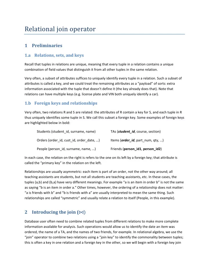
Recall that tuples in relations are unique, meaning that every tuple in a relation contains a unique combination of field values that distinguish it from all other tuples in the same relation. Very often, a subset of attributes suffices to uniquely identify every tuple in a relation. Such a subset of attributes is called a key, and we could treat the remaining attributes as a “payload” of sorts: extra information associated with the tuple that doesn’t define it (the key already does that). Note that relations can have multiple keys (e.g. license plate and VIN both uniquely identify a car).

1.b Foreign keys and relationships

Very often, two relations R and S are related: the attributes of R contain a key for S, and each tuple in R thus uniquely identifies some tuple in S. We call this subset a foreign key. Some examples of foreign keys are highlighted below in bold: Students (student_id, surname, name) TAs (student_id, course, section) Orders (order_id, cust_id, order_date, …) Items (order_id, part_num, qty, …) People (person_id, surname, name, …) Friends (person_id1, person_id2) In each case, the relation on the right is refers to the one on its left by a foreign key; that attribute is called the “primary key” in the relation on the left. Relationships are usually asymmetric: each item is part of an order, not the other way around; all teaching assistants are students, but not all students are teaching assistants, etc. In these cases, the tuples (a,b) and (b,a) have very different meanings. For example “a is an item in order b” is not the same as saying “b is an item in order a.” Other times, however, the ordering of a relationship does not matter: “a is friends with b” and “b is friends with a” are usually interpreted to mean the same thing. Such relationships are called “symmetric” and usually relate a relation to itself (People, in this example).

2 Introducing the join (⨝

Database user often need to combine related tuples from different relations to make more complete information available for analysis. Such operations would allow us to identify the date an item was

• rdered, the name of a TA, and the names of two friends, for example. In relational algebra, we use the

“join” operator to combine two relations using a “join key” to identify the commonality between tuples; this is often a key in one relation and a foreign key in the other, so we will begin with a foreign key join

and later expand it to more general cases. If R is a set of tuples that contain the foreign key, and S is a dictionary mapping keys to payloads in S, a naïve python function performing a foreign key join might look something like this:

def join1(R, get_fk, S): for r in R: try: yield r + S[get_fk(r)] except KeyError: pass

There are several things to note here:

• 1. The key occurs in both input tuples, but we only include it once in the output tuple.
• 2. Tuples from either input having no matches are silently discarded. We’ll revisit this later.
• 3. The relational join operator is commutative, but our toy is not. More on this later as well.
• 4. The above code only works for relations having a foreign key relationship; we can relax the

definition of a join key in several useful ways that the above code cannot express.

• 5. Join is set‐oriented (like nearly all RA operators), so the DBMS has a lot of flexibility in choosing

how to implement it. A good half‐dozen basic join algorithms exist, with a vast number of minor variants; join1() is suitable for foreign key joins when S is a dictionary that fits in memory.

2.a Natural join

Relational algebra requires both relations to use the same name for each attribute in the join key, because the latter is defined as the intersection of the input schemata; the output schema is similarly defined as the union of input schemata. This arrangement is called a “natural” join, denoted by the bowtie symbol: ⨝. The input schemata often don’t match in practice, however, so natural join is both error‐prone (the join key can easily contain the wrong attributes) and “brittle” (adding or renaming an attribute can break queries that do not mention that attribute). The most common problem arises when unrelated attributes happen to have the same name and become part of the join key when they should be treated as part of the payload instead. Unless a natural join is requested specially, SQL requires queries to specify join keys explicitly, by stating which attributes from the input relations should match.

2.b Join is commutative

The relational join operator is commutative (R ⨝ S = S ⨝ R). Unfortunately, this is not true for our simple python code: It would work just fine if we joined R=items and S=orders, but would break badly if we tried to join R=orders and S=items. The reason is simple: the foreign key (items.order_id) guarantees that every item points to at most one order, but any number of items might point to a given order.1 We would therefore either lose tuples while building the dictionary S=items (if S forbids duplicates), or encounter collisions while probing with R=orders (if S allows duplicates). Either way, the resulting relation would contain only one item per order, which is clearly wrong. It’s tempting to just switch R and

1 In fact, that’s probably the main reason order and items are separate in the first place!

S internally so R always contains the foreign key and S always contains the dictionary, but that’s not a general solution:  R might be an iterator over a stream of data that’s too large to fit in memory, so we couldn’t easily store (“materialize”) it into the (hash‐based, memory‐resident) dictionary the join1() algorithm requires for S.  We’ll see later that foreign keys are not the only possible “join key” allowed, and that the “join key” need not be a key in either R or S. It would then be difficult or impossible to build a suitable dictionary without allowing duplicates.  It turns out that key equality is not the only useful matching policy, so we may not be able to build a dictionary at all (we’ll come back to this in the next section). In order for join to become both commutative and general purpose, we will have to stop assuming S is keyed off the foreign key we extract from R. An updated python snippet might look like this:2

def join2(R, rsplit, S, ssplit): for rk,rpayload in (rsplit(r) for r in R): for sk,spayload in (ssplit(s) for s in S): if rk == sk: yield rpayload + rk + spayload

This time, we check for all possible matches of either side against the other, so it doesn’t matter which relation is R vs. S. As a nice side effect, we’ve also made explicit the concept of a “join key” that can be an arbitrary subset of attributes (not necessarily a key) common to both R and S. As before, the join key is the same on both sides, so we choose to only include it once in the output.

2.c Left outer join

Recall that the basic join algorithms in Sections 2 and 3 silently discard tuples from R unless they match a tuple in S; unreferenced tuples in S are also discarded. This is a consequence of the formal definition of join – and it’s often the “right” thing to do – but sometimes this information loss is undesirable. Suppose, for example, we wanted to find the total sales for every product in the catalog. Products having no sales at all would not be reported, because the join would only preserve those products appearing in some sales order.3 Going back to our naïve join1() algorithm, the solution is pretty straightforward if R is the product relation. We simply designate a “fake” s‐tuple to use whenever we can’t find a real s‐tuple to join with:

def join3(R, get_fk, S, fake_s): for r in R: try: yield r + S[get_fk (r)] except KeyError: yield r + fake_s

2 This is the join equivalent of a bubble sort: really simple, but so frightfully inefficient that database engines

almost never stoop to using it; if you’re interested in studying efficient join algorithms, take D43.

3 It’s far less likely to happen, but a sales order with no items would also be lost during the join

This is called a “left outer join” or just “left join” (⟕ or ⨝L), because every tuple on the left relation (R, in our case) will appear in the join’s output even if doesn’t match any tuples in S (e.g. it can return tuples “outside” the set of tuples a join would normally return). A similar “right outer join” (⟖ or ⨝R) can be defined, or even a “full outer join” (⟗ or ⨝O) that returns every tuple from both the left and right

• relation. However, the code for those is a lot uglier, so I won’t give an example here.4 In theory, the user

can supply any value they wish for the fields of a fake tuple, but in practice database engines usually provide the special value NULL, which is nothing and is not equal to anything (not even itself); applications can test for and replace NULL values later as desired. Finally, it is important to note that left and right outer joins do *not* commute! In other words, R ⟕ S ≠ S ⟕ R, though it *is* true that R ⟕ S = S ⟖ R. Further, outer joins do not always obey the associative property when mixed with natural joins: (R ⟕ S) ⨝ T ≠ R ⟕ (S ⨝ T).5

3 Equijoin, Cartesian products, and intersection

As we hinted earlier, the commutative version of our join algorithm is actually more general than a mere “foreign key” join: it can use any subset of attributes shared by the two relations, and that subset need not be a key in either relation. Mathematically, it turns out that joins are just a Cartesian product followed by selection: enumerate all possible pairwise combinations of tuples from R and S, and throw away any results whose join keys don’t match. The join3() algorithm in Section 3 does exactly this, and it’s shockingly inefficient for large inputs because almost none of the combinations actually match.

Figure 1. Join as selection over a Cartesian product

4 Ugly enough, it turns out, that several database engines support only left outer join 5 Can you think of any examples where associativity does and does not hold?

c e f a b d d f c e a b

⨝

a a a a a e c d f f f f b e f d b b b b b a b e c f a a b f

. . .

f f a c

   

b d



Next, let’s see what happens if we partition R and S on the join key, placing into groups all tuples having the same join key value.6 For each partition in S, only one partition in R can possibly satisfy the join predicate, namely, the one having the same join key; there’s no point in evaluating mismatched R/S pairs, because the selection that follows is guaranteed to eliminate them anyway. The join can therefore be expressed by computing the Cartesian product for each matching R/S partition pair, then returning the union of all resulting sets of tuples:

Figure 2 Join as a union of Cartesian products

This construction leads to a number of useful observations about the behavior of joins:7  Joins never create new partitions: the output contains only partitions that exist in both R and S  The cardinality of a join’s output is called “join cardinality” and may be larger or smaller than the input cardinalities.  Output partitions have cardinality equal to the product of cardinalities of the corresponding input partitions, and quickly become very large if a large partition in R matches a large partition in S.  Foreign key joins output at most one tuple for each tuple in the foreign key relation, because each partition in the primary key relation contains only a single tuple (= no change in cardinality, the relational algebra equivalent to multiplying a number by one).  Lost tuples are due to unmatched partitions (those existing in only one of R or S).  Outer joins can be achieved by padding tuples from unmatched partitions and including them in the union of Cartesian products.

3.a Join, intersection, and Cartesian product

It turns out that join, intersection and Cartesian product are quite closely related: the latter two

• perators are just degenerate joins! Recall that the natural join combines two relations that have

partially overlapping schemata, with the overlapping part becoming the join key. We just saw that the

6 There can be any number of tuples in a given partition, unless the join key is also a key for that relation 7 It also suggests an highly efficient – and widely used – algorithm for performing equijoins in O(|R|+|S|) time

e d a d e f b c f b c a

⨯ ⨯ ⨯

d b d e f c a f b d e f a c c a a a

worst case is the empty join key (= non‐overlapping schemata), which results in a Cartesian product of the two relations. At the other extreme, the join key is the schema for both relations, meaning that all partitions have cardinality one; in this case the join condition is tuple equality, and the only question is whether a given tuple exists in both relations. Set intersection, in other words! Relaxing that condition slightly so that the join key is a superkey8 in both relations gives something very like intersection, with 1:1 matches of input tuples and output tuples containing all attributes found in either input. The only difference is that the output tuples contain the “payload” columns from both relations. The relationship between intersection, join, and Cartesian product was noted just a few years after Codd introduced relational algebra, and join is sometimes called “generalized intersection.” Graphically, we might depict the relationship in schemata as follows: In all cases, the result is the union over Cartesian products of partitions, where each partition contains tuples with the same value of join key, as illustrated in Figure 2.9

3.b Join is associative

Join is a binary operator, taking two input relations and producing a third as output. To join three or more relations requires chaining multiple join operations together. Because of the way partitions are formed, join is associative (R ⨝ S) ⨝ T = R ⨝ (S ⨝ T): partitions by definition do not overlap or interfere with each other, and Cartesian product within a partition is associative: (A x B) ⨯ C = A ⨯ (B ⨯ C). That said, however, evaluation order can have a huge impact on how long the operation takes. Imagine, for example, joining a very large partition in R with a very large partition in S, only to discover that the resulting enormous partition is actually unmatched in T! The database query optimizer works very hard to avoid such situations, in general by first performing those joins that involve smaller relations or for which internal statistics predict low join cardinality.

3.c Theta join

Having made the leap from foreign key join to equijoin, it’s natural to wonder whether we can replace the key equality predicate with some inequality (‘>’, ‘<=’, etc.), or even a general predicate over the

8 A superkey is any set of columns that includes a key, just like a superset is to a set. 9 It’s interesting to compare generalized intersection with generalized union. Where the relation produced by

generalized intersection conceptually involves selection and has a schema that is the union of the two input schemata, generalized union conceptually involves projection and produces a relation whose schema is the intersection of input schemata. Nobody seems to know what to make of this odd duality.

Intersection (full overlap) Natural join (partial overlap) Cartesian product (no overlap)

entire tuple. The short answer is “yes, absolutely!” Formally it’s called a theta join, and it’s not terribly hard to understand. I’ll just point out a few things:  Although the concept of “partitions” still applies, theta joins may allow one partition in R to match multiple partitions in S (and one partition in S to match several in R as well). This can lead to larger result sets, sometimes significantly so (the bad case is the ‘!=’ predicate, which usually matches).  Most theta joins can be expressed as equijoin followed by selection. It’s usually easier to reason about the latter, but the math is equivalent so it’s a matter of preference which to use.  Predicates in theta joins always involve attributes from both input relations; predicates involving

• nly attributes of one input are normal selections.

3.d Self‐join

One common and particularly useful theta join sets S=R and has the join predicate p(k1,k2) = k1 < k2, where k1 and k2 are the keys of arbitrary tuples in R; the resulting “self‐join” enumerates all unique pairwise combinations of tuples in R, which is very helpful when working with symmetric relationships that treat (A,B) and (B,A) as equivalent.