Reinforcement Learning (RL) CE-717: Machine Learning Sharif - PowerPoint PPT Presentation
Reinforcement Learning (RL) CE-717: Machine Learning Sharif University of Technology M. Soleymani Fall 2018 Most slides have been taken from Klein and Abdeel, CS188, UC Berkeley. Reinforcement Learning (RL) Learning as a result of
MDP: Optimal policy state-value and action-value functions Optimal policies share the same optimal state-value function ( 𝑊 𝜌 ∗ (𝑡) will be abbreviated as 𝑊 ∗ (𝑡) ): 𝑊 ∗ 𝑡 = max 𝑊 𝜌 𝑡 , ∀𝑡 ∈ 𝑇 𝜌 And the same optimal action-value function: 𝑅 ∗ 𝑡, 𝑏 = max 𝑅 𝜌 𝑡, 𝑏 , ∀𝑡 ∈ 𝑇, 𝑏 ∈ (𝑡) 𝜌 For any MDP, a deterministic optimal policy exists! 28
Optimal policy If we have 𝑊 ∗ (𝑡) and 𝑄(𝑡 𝑢+1 |𝑡 𝑢 , 𝑏 𝑢 ) we can compute 𝜌 ∗ (𝑡) 𝜌 ∗ 𝑡 = argmax 𝑏 𝑏 + 𝛿𝑊 ∗ (𝑡′) 𝒬 𝑡𝑡 ′ ℛ 𝑡𝑡 ′ 𝑏 𝑡 ′ It can also be computed as: 𝜌 ∗ 𝑡 = argmax 𝑅 ∗ 𝑡, 𝑏 𝑏∈(𝑡) Optimal policy has the interesting property that it is the optimal policy for all states. Share the same optimal state-value function It is not dependent on the initial state. use the same policy no matter what the initial state of MDP is 29
Bellman optimality equation 𝑊 ∗ 𝑡 = max + 𝛿𝑊 ∗ 𝑡′ 𝑏 𝑏 𝑏∈(𝑡) 𝒬 𝑡𝑡 ′ ℛ 𝑡𝑡 ′ 𝑡 ′ 𝑅 ∗ 𝑡, 𝑏 = 𝑏 ′ 𝑅 ∗ 𝑡 ′ , 𝑏 ′ 𝑏 𝑏 𝒬 𝑡𝑡 ′ ℛ 𝑡𝑡 ′ + 𝛿 max 𝑡 ′ 𝑊 ∗ 𝑡 = max 𝑏∈(𝑡) 𝑅 ∗ 𝑡, 𝑏 𝑅 ∗ 𝑡, 𝑏 = + 𝛿𝑊 ∗ 𝑡′ 𝑏 𝑏 𝒬 𝑡𝑡 ′ ℛ 𝑡𝑡 ′ 𝑡 ′ 30
Optimal Quantities The value (utility) of a state s: V * (s) = expected utility starting in s and acting optimally s is a s state a The value (utility) of a q-state (s,a): (s, a) is a s, a Q * (s,a) = expected utility starting out q-state having taken action a from state s and s,a,s ’ (s,a,s ’ ) is a (thereafter) acting optimally transition s ’ The optimal policy: * (s) = optimal action from state s 31
Snapshot of Demo – Gridworld V Values Noise = 0.2 Discount = 0.9 Living reward = 0 32
Snapshot of Demo – Gridworld Q Values Noise = 0.2 Discount = 0.9 Living reward = 0 33
Value Iteration algorithm Consider only MDPs with finite state and action spaces: Initialize all 𝑊(𝑡) to zero 1) Repeat until convergence 2) for 𝑡 ∈ 𝑇 𝑏 𝑏 σ 𝑡 ′ 𝒬 𝑡𝑡 ′ 𝑊(𝑡) ← max ℛ 𝑡𝑡 ′ + 𝛿𝑊(𝑡′) 𝑏 for 𝑡 ∈ 𝑇 3) 𝑏 𝑏 σ 𝑡 ′ 𝒬 𝑡𝑡 ′ 𝜌(𝑡) ← argmax ℛ 𝑡𝑡 ′ + 𝛿𝑊(𝑡′) 𝑏 𝑊(𝑡) converges to 𝑊 ∗ (𝑡) Asynchronous: Instead of updating values for all states at once in each iteration, it can update them state by state, or more often to some states than others. 34
Value Iteration Bellman equations characterize the optimal values: V(s) a s, a s,a,s Value iteration computes them: ’ V(s ’ ) Value iteration is just a fixed point solution method … though the V k vectors are also interpretable as time-limited values 35
V k+1 (s) a Racing Search Tree s, a s,a,s ’ V k (s ’ ) 36
Racing Search Tree 37
Time-Limited Values Key idea: time-limited values Define V k (s) to be the optimal value of s if the game ends in k more time steps 38
Value Iteration Start withV 0 (s) = 0: no time steps left means an expected reward sum of zero Given vector ofV k (s) values, do one ply of expectimax from each state: V k+1 (s) a s, a Repeat until convergence s,a,s ’ V k (s ’ ) Complexity of each iteration: O(S 2 A) Theorem: will converge to unique optimal values Basic idea: approximations get refined towards optimal values Policy may converge long before values do 39
Example: Value Iteration 3.5 2.5 0 2 1 0 Assume no discount! 0 0 0 40
Computing Time-Limited Values 41
k=0 Noise = 0.2 Discount = 0.9 Living reward = 0 42
k=1 Noise = 0.2 Discount = 0.9 Living reward = 0 43
k=2 Noise = 0.2 Discount = 0.9 Living reward = 0 44
k=3 Noise = 0.2 Discount = 0.9 Living reward = 0 45
k=4 Noise = 0.2 Discount = 0.9 Living reward = 0 46
k=5 Noise = 0.2 Discount = 0.9 Living reward = 0 47
k=6 Noise = 0.2 Discount = 0.9 Living reward = 0 48
k=7 Noise = 0.2 Discount = 0.9 Living reward = 0 49
k=8 Noise = 0.2 Discount = 0.9 Living reward = 0 50
k=9 Noise = 0.2 Discount = 0.9 Living reward = 0 51
k=10 Noise = 0.2 Discount = 0.9 Living reward = 0 52
k=11 Noise = 0.2 Discount = 0.9 Living reward = 0 53
k=12 Noise = 0.2 Discount = 0.9 Living reward = 0 54
k=100 Noise = 0.2 Discount = 0.9 Living reward = 0 55
Computing Actions from Values Let ’ s imagine we have the optimal valuesV*(s) How should we act? It ’ s not obvious! We need to do (one step) This is called policy extraction, since it gets the policy implied by the values 56
Computing Actions from Q-Values Let ’ s imagine we have the optimal q-values: How should we act? Completely trivial to decide! Important lesson: actions are easier to select from q-values than values! 57
Convergence* How do we know the V k vectors are going to converge? Case 1: If the tree has maximum depth M, then V M holds the actual untruncated values Case 2: If the discount is less than 1 Sketch: For any state V k and V k+1 can be viewed as depth k+1 results in nearly identical search trees The difference is that on the bottom layer, V k+1 has actual rewards while V k has zeros That last layer is at best all R MAX It is at worst R MIN But everything is discounted by γ k that far out So V k and V k+1 are at most γ k max|R| different So as k increases, the values converge 58
Value Iteration Value iteration works even if we randomly traverse the environment instead of looping through each state and action (update asynchronously) but we must still visit each state infinitely often Value Iteration It is time and memory expensive 59
Problems with Value Iteration Value iteration repeats the Bellman updates: s a Problem 1: It ’ s slow – O(S 2 A) per iteration s, a s,a,s ’ Problem 2: The “ max ” at each state rarely changes s ’ Problem 3: The policy often converges long before the values 60
Convergence [Russel, AIMA, 2010] 61
Main steps in solving Bellman optimality equations Two kinds of steps, which are repeated in some order for all the states until no further changes take place 𝑏 𝑏 + 𝛿𝑊 𝜌 (𝑡′) 𝜌 𝑡 = argmax 𝒬 𝑡𝑡 ′ ℛ 𝑡𝑡 ′ 𝑏 𝑡 ′ 𝜌(𝑡) ℛ 𝑡𝑡 ′ 𝜌(𝑡) + 𝛿𝑊 𝜌 (𝑡′) 𝑊 𝜌 𝑡 = 𝒬 𝑡𝑡 ′ 𝑡 ′ 62
Policy Iteration algorithm Initialize 𝜌(𝑡) arbitrarily 1) Repeat until convergence 2) Compute the value function for the current policy 𝜌 (i.e. 𝑊 𝜌 ) 𝑊 ← 𝑊 𝜌 for 𝑡 ∈ 𝑇 𝑏 𝑏 σ 𝑡 ′ 𝒬 𝑡𝑡 ′ 𝜌(𝑡) ← argmax ℛ 𝑡𝑡 ′ + 𝛿𝑊(𝑡′) 𝑏 updates the policy (greedily) using the current value function. 𝜌(𝑡) converges to 𝜌 ∗ (𝑡) 63
Policy Iteration Repeat steps until policy converges Step 1: Policy evaluation: calculate utilities for some fixed policy (not optimal utilities!) until convergence Step 2: Policy improvement: update policy using one-step look-ahead with resulting converged (but not optimal!) utilities as future values This is policy iteration It ’ s still optimal! Can converge (much) faster under some conditions 64
Fixed Policies Evaluation Do what says to do Do the optimal action s s (s) a s, (s) s, a s, (s),s ’ s,a,s ’ s ’ s ’ fixed some policy (s), then the tree max over all actions to compute the optimal values would be simpler – only one action per state 65
Utilities for a Fixed Policy Another basic operation: compute the utility of a state s s under a fixed (generally non-optimal) policy (s) s, (s) Recursive relation (one-step look-ahead / Bellman equation): s, (s),s ’ s ’ V (s) = expected total discounted rewards starting in s and following 66
Policy Evaluation How do we calculate the V ’ s for a fixed policy ? Idea 1: Turn recursive Bellman equations into updates s (like value iteration) (s) s, (s) s, (s),s ’ s ’ Efficiency: O(S 2 ) per iteration Idea 2: Without the maxes, the Bellman equations are just a linear system 67
Policy Iteration Evaluation: For fixed current policy , find values with policy evaluation: Iterate until values converge: Improvement: For fixed values, get a better policy using policy extraction One-step look-ahead: 68
When to stop iterations: [Russel, AIMA 2010] 69
Comparison Both value iteration and policy iteration compute the same thing (all optimal values) In value iteration: Every iteration updates both the values and (implicitly) the policy We don ’ t track the policy, but taking the max over actions implicitly recomputes it In policy iteration: We do several passes that update utilities with fixed policy (each pass is fast because we consider only one action, not all of them) After the policy is evaluated, a new policy is chosen (slow like a value iteration pass) The new policy will be better (or we ’ re done) Both are dynamic programs for solving MDPs 70
MDP Algorithms: Summary So you want to … . Compute optimal values: use value iteration or policy iteration Compute values for a particular policy: use policy evaluation Turn your values into a policy: use policy extraction (one-step lookahead) 71
Unknown transition model 𝑏 So far: learning optimal policy when we know 𝒬 𝑡𝑡 ′ (i.e. T(s,a,s ’ ) ) and ℛ 𝑡𝑡 ′ 𝑏 it requires prior knowledge of the environment's dynamics If a model is not available, then it is particularly useful to estimate action values rather than state values 72
Reinforcement Learning Still assume a Markov decision process (MDP): A set of states s S A set of actions (per state) A A model T(s,a,s ’ ) A reward function R(s,a,s ’ ) Still looking for a policy (s) New twist: don ’ t know T or R I.e. we don ’ t know which states are good or what the actions do Must actually try actions and states out to learn 73
Reinforcement Learning Agent State: s Actions: a Reward: r Environmen t Basic idea: Receive feedback in the form of rewards Agent ’ s utility is defined by the reward function Must (learn to) act so as to maximize expected rewards All learning is based on observed samples of outcomes! 74
Applications Control & robotics Autonomous helicopter self-reliant agent must do to learn from its own experiences. eliminating hand coding of control strategies Board games Resource (time, memory, channel, … ) allocation 75
Double Bandits 76
Let ’ s Play! $2 $2 $0 $2 $2 $2 $2 $0 $0 $0 77
What Just Happened? That wasn ’ t planning, it was learning! Specifically, reinforcement learning There was an MDP, but you couldn ’ t solve it with just computation You needed to actually act to figure it out Important ideas in reinforcement learning that came up Exploration: you have to try unknown actions to get information Exploitation: eventually, you have to use what you know Regret: even if you learn intelligently, you make mistakes Sampling: because of chance, you have to try things repeatedly Difficulty: learning can be much harder than solving a known MDP 78
Offline (MDPs) vs. Online (RL) Offline Solution Online Learning 79
RL algorithms Model-based (passive) Learn model of environment (transition and reward probabilities) Then, value iteration or policy iteration algorithms Model-free (active) 80
Model-Based Learning Model-Based Idea: Learn an approximate model based on experiences Solve for values as if the learned model were correct Step 1: Learn empirical MDP model Count outcomes s ’ for each s, a Normalize to give an estimate of Discover each when we experience (s, a, s ’ ) Step 2: Solve the learned MDP For example, use value iteration, as before 81
Example: Model-Based Learning Input Policy Observed Episodes (Training) Learned Model Episode 1 Episode 2 T(s,a,s ’ ). T(B, east, C) = 1.00 B, east, C, -1 B, east, C, -1 A T(C, east, D) = 0.75 C, east, D, -1 C, east, D, -1 T(C, east, A) = 0.25 D, exit, x, +10 D, exit, x, +10 … B C D R(s,a,s ’ ). Episode 3 Episode 4 E R(B, east, C) = -1 E, north, C, -1 E, north, C, -1 R(C, east, D) = -1 C, east, D, -1 C, east, A, -1 R(D, exit, x) = +10 Assume: = 1 D, exit, x, +10 A, exit, x, -10 … 82
Model-Free Learning 83
Reinforcement Learning We still assume an MDP: A set of states s S A set of actions (per state) A A modelT(s,a,s ’ ) A reward function R(s,a,s ’ ) Still looking for a policy (s) New twist: don ’ t knowT or R, so must try out actions Big idea: Compute all averages over T using sample outcomes 84
Direct Evaluation of a Policy Goal: Compute values for each state under Idea:Average together observed sample values Act according to Every time you visit a state, write down what the sum of discounted rewards turned out to be Average those samples This is called direct evaluation 85
Example: Direct Evaluation Input Policy Observed Episodes (Training) Output Values Episode 1 Episode 2 -10 B, east, C, -1 B, east, C, -1 A A C, east, D, -1 C, east, D, -1 D, exit, x, +10 D, exit, x, +10 +8 +4 +10 B C D B C D Episode 3 Episode 4 -2 E E E, north, C, -1 E, north, C, -1 C, east, D, -1 C, east, A, -1 Assume: = 1 D, exit, x, +10 A, exit, x, -10 86
Monte Carlo methods do not assume complete knowledge of the environment require only experience sample sequences of states, actions, and rewards from on-line or simulated interaction with an environment are based on averaging sample returns are defined for episodic tasks 87
A Monte Carlo control algorithm using exploring starts Initialize 𝑅 and 𝜌 arbitrarily and 𝑆𝑓𝑢𝑣𝑠𝑜𝑡 to empty lists 1) Repeat 2) Generate an episode using 𝜌 and exploring starts for each pair of 𝑡 and 𝑏 appearing in the episode 𝑆 ← return following the first occurrence of 𝑡, 𝑏 Append 𝑆 to 𝑆𝑓𝑢𝑣𝑠𝑜𝑡(𝑡, 𝑏) 𝑅 𝑡, 𝑏 ← 𝑏𝑤𝑓𝑠𝑏𝑓 𝑆𝑓𝑢𝑣𝑠𝑜𝑡(𝑡, 𝑏) for each 𝑡 in the episode 𝜌(𝑡) ← argmax 𝑅(𝑡, 𝑏) 𝑏 88
Problems with Direct Evaluation Output Values What ’ s good about direct evaluation? It ’ s easy to understand -10 A It doesn ’ t require any knowledge of T, R +8 +4 +10 It eventually computes the correct average B C D values, using just sample transitions -2 E What bad about it? If B and E both go to C It wastes information about state connections under this policy, how can Each state must be learned separately their values be different? So, it takes a long time to learn 89
Connections between states Simplified Bellman updates calculate V for a fixed policy: s Each round, replace V with a one-step-look-ahead layer over V (s) s, (s) s, (s),s ’ s ’ This approach fully exploited the connections between the states Unfortunately, we need T and R to do it! Key question: how can we do this update to V without knowing T and R? In other words, how to we take a weighted average without knowing the weights? 90
Connections between states We want to improve our estimate of V by computing these averages: Idea: Take samples of outcomes s ’ (by doing the action!) and average s (s) s, (s) s, (s),s ’ s 1 s s 2 s 3 ' ' ' ' Almost! But we can ’ t rewind time to get sample after sample from state s. 91
Temporal Difference Learning Big idea: learn from every experience! Update V(s) each time we experience a transition (s, a, s ’ , r) s Likely outcomes s ’ will contribute updates more often (s) s, (s) Temporal difference learning of values Policy still fixed, still doing evaluation! Move values toward value of whatever successor occurs: running s ’ average Sample of V(s): Update to V(s): Same update: 92
Exponential Moving Average Exponential moving average The running interpolation update: Makes recent samples more important: Forgets about the past (distant past values were wrong anyway) Decreasing learning rate (alpha) can give converging averages 93
Example: Temporal Difference Learning States Observed Transitions B, east, C, -2 C, east, D, -2 A 0 0 0 B C D 0 0 -1 0 -1 3 8 8 8 E 0 0 0 Assume: = 1, α = 1/2 94
Temporal difference methods TD learning is a combination of MC and DP ) i.e. Bellman equations) ideas. Like MC methods, can learn directly from raw experience without a model of the environment's dynamics. Like DP , update estimates based in part on other learned estimates, without waiting for a final outcome. 95
Temporal difference on value function 𝑊 𝑡 𝑢 ← 𝑊 𝑡 𝑢 + 𝛽 𝑠 𝑢+1 + 𝛿𝑊 𝑡 𝑢+1 − 𝑊(𝑡 𝑢 ) 𝜌 : the policy to be evaluated Initialize 𝑊(𝑡) arbitrarily 1) Repeat (for each episode) 2) Initialize s 𝑏 ← action given by policy 𝜌 for 𝑡 Take action 𝑏 ; observe reward 𝑠 , and next state 𝑡′ 𝑊 𝑡 ← 𝑊 𝑡 + 𝛽 𝑠 + 𝛿𝑊 𝑡′ − 𝑊(𝑡) until s is terminal fully incremental fashion 96
Problems with TD Value Learning TD value leaning is a model-free way to do policy evaluation, mimicking Bellman updates with running sample averages However, if we want to turn values into a (new) policy, we ’ re sunk: s a s, a s,a,s ’ s ’ 97
Unknown transition model: New policy With a model, state values alone are sufficient to determine a policy simply look ahead one step and chooses whichever action leads to the best combination of reward and next state Without a model, state values alone are not sufficient. However, if agent knows 𝑅(𝑡, 𝑏) , it can choose optimal action without knowing 𝑈 and 𝑆 : 𝜌 ∗ 𝑡 = argmax 𝑅(𝑡, 𝑏) 𝑏 98
Unknown transition model: New policy Idea: learn Q-values, not state values Makes action selection model-free too! 99
Detour: Q-Value Iteration Value iteration: find successive (depth-limited) values Start with V 0 (s) = 0, which we know is right Given V k , calculate the depth k+1 values for all states: But Q-values are more useful, so compute them instead Start with Q 0 (s,a) = 0, which we know is right Given Q k , calculate the depth k+1 q-values for all q-states: 100
Recommend
More recommend
Explore More Topics
Stay informed with curated content and fresh updates.
