Reinforcement Learning Part 2 CS 760@UW-Madison Goals for the - PowerPoint PPT Presentation
Reinforcement Learning Part 2 CS 760@UW-Madison Goals for the lecture you should understand the following concepts value functions and value iteration (review) Q functions and Q learning (review) exploration vs. exploitation
Reinforcement Learning Part 2 CS 760@UW-Madison
Goals for the lecture you should understand the following concepts • value functions and value iteration (review) • Q functions and Q learning (review) • exploration vs. exploitation tradeoff • compact representations of Q functions • reinforcement learning example 2
Value function for a policy • given a policy π : S → A define = t ( ) [ ] assuming action sequence chosen V s E r t according to π starting at state s = 0 t we want the optimal policy π * where • p * = argmax p V p ( s ) for all s we’ll denote the value function for this optimal policy as V * ( s ) 3
Value iteration for learning V * ( s ) initialize V ( s ) arbitrarily loop until policy good enough { loop for s ∈ S { loop for a ∈ A { + ( , ) ( , ) ( ' | , ) ( ' ) Q s a r s a P s s a V s ' s S } ( ) max ( , ) V s Q s a a } } 4
Q learning define a new function, closely related to V* + * * * ( ) ( , ( )) ( ' ) V s E r s s E V s * ' | , ( ) s s s + * ( , ) ( , ) ( ' ) Q s a E r s a E V s ' | , s s a if agent knows Q ( s, a ) , it can choose optimal action without knowing P ( s’ | s , a ) * * ( ) arg max ( , ) ( ) max ( , ) s Q s a V s Q s a a a and it can learn Q ( s, a ) without knowing P ( s ’ | s , a ) 5
Q learning for deterministic worlds ˆ ( , ) 0 for each s, a initialize table entry Q s a observe current state s do forever select an action a and execute it receive immediate reward r observe the new state s ’ update table entry ˆ ˆ + ( , ) max ( ' , ' ) Q s a r Q s a ' a s ← s ’ 6
Q learning for nondeterministic worlds ˆ for each s, a initialize table entry ( , ) 0 Q s a observe current state s do forever select an action a and execute it receive immediate reward r observe the new state s ’ update table entry ˆ ˆ ˆ − + + ( , ) ( 1 ) ( , ) max ( ' , ' ) Q s a Q s a r Q s a − − 1 ' 1 n n n n a n s ← s ’ where α n is a parameter dependent 1 a n = on the number of visits to the given 1 + visits n ( s , a ) ( s, a ) pair 7
Q’ s vs. V’ s Q V V Q V • Which action do we choose when we’re in a given state? • V’ s (model-based) • need to have a ‘next state’ function to generate all possible states • choose next state with highest V value. • Q’ s (model-free) • need only know which actions are legal • generally choose next state with highest Q value. 8
Exploration vs. Exploitation • in order to learn about better alternatives, we shouldn’t always follow the current policy (exploitation) • sometimes, we should select random actions (exploration) • one way to do this: select actions probabilistically according to: ˆ ( , ) Q s a c i = ( | ) P a s ˆ i ( , ) Q s a c j j where c > 0 is a constant that determines how strongly selection favors actions with higher Q values 9
Q learning with a table As described so far, Q learning entails filling in a huge table states s 0 s 1 s 2 . . . s n . a 1 . a 2 . A table is a very a 3 Q ( s 2 , a 3 ) actions . . . verbose way to . represent a function . . a k 10
Representing Q functions more compactly We can use some other function representation (e.g. a neural net) to compactly encode a substitute for the big table Q ( s, a 1 ) Q ( s, a 2 ) encoding of the state ( s ) Q ( s, a k ) e ach input unit encodes o r could have one net a property of the state for each possible action (e.g., a sensor value) 11
Why use a compact Q function? Full Q table may not fit in memory for realistic problems 1. 2. Can generalize across states, thereby speeding up convergence i.e. one instance ‘fills’ many cells in the Q table Notes When generalizing across states, cannot use α =1 1. Convergence proofs only apply to Q tables 2. 3. Some work on bounding errors caused by using compact representations (e.g. Singh & Yee, Machine Learning 1994) 12
Q tables vs. Q nets Given: 100 Boolean-valued features 10 possible actions Size of Q table 10 × 2 100 entries Size of Q net (assume 100 hidden units) 100 × 100 + 100 × 10 = 11,000 weights weights between weights between inputs and HU’s HU’s and outputs 13
Representing Q functions more compactly • we can use other regression methods to represent Q functions k -NN regression trees support vector regression etc. 14
Q learning with function approximation measure sensors, sense state s 0 1. ˆ Q n ( s 0 , a ) predict for each action a 2. select action a to take (with randomization to ensure 3. exploration) apply action a in the real world 4. sense new state s 1 and immediate reward r 5. ˆ Q n ( s 1 , a ') calculate action a’ that maximizes 6. 7. train with new instance = s x 0 ˆ ˆ − + + ( 1 ) ( , ) max ( , ' ) y Q s a r Q s a 0 ' 1 a Calculate Q-value you would have put into Q-table, and use it as the training label 15
ML example: reinforcement learning to control an autonomous helicopter video of Stanford University autonomous helicopter from http://heli.stanford.edu/ 16
Stanford autonomous helicopter sensing the helicopter’s state • orientation sensor accelerometer rate gyro magnetometer • GPS receiver (“2cm accuracy as long as its antenna is pointing towards the sky”) • ground-based cameras actions to control the helicopter
Experimental setup for helicopter 1. Expert pilot demonstrates the airshow several times 2. Learn a reward function based on desired trajectory 3. Learn a dynamics model 4. Find the optimal control policy for learned reward and dynamics model 5. Autonomously fly the airshow 6. Learn an improved dynamics model. Go back to step 4
Learning dynamics model P ( s t+1 | s t , a ) • state represented by helicopter’s ( ) x , y , z position velocity ( ) w x , w y , w z angular velocity • action represented by manipulations of 4 controls ( ) u 1 , u 2 , u 3 , u 4 • dynamics model predicts accelerations as a function of current state and actions • accelerations are integrated to compute the predicted next state
Learning dynamics model P ( s t+1 | s t , a ) dynamics model • A, B, C, D represent model parameters • g represents gravity vector w ’s are random variables representing noise and unmodeled effects • • l inear regression task!
Learning a desired trajectory • repeated expert demonstrations are often suboptimal in different ways • given a set of M demonstrated trajectories k s = = − = − j k for 0 ,..., 1 , 0 ,..., 1 y j N k M j k u j action on j th step of trajectory k state on j th step of trajectory k • try to infer the implicit desired trajectory * s = = t for 0 z t ,...,H t * u t
Learning a desired trajectory colored lines: demonstrations of two loops black line: inferred trajectory Figure from Coates et al., CACM 2009
Learning reward function • EM is used to infer desired trajectory from set of demonstrated trajectories • The reward function is based on deviations from the desired trajectory
Finding the optimal control policy • finding the control policy is a reinforcement learning task * arg max ( , ) | E r s t a t • RL learning methods described earlier don’t quite apply because state and action spaces are both continuous • A special type of Markov decision process in which the optimal policy can be found efficiently • reward is represented as a linear function of state and action vectors • next state is represented as a linear function of current state and action vectors • They use an iterative approach that finds an approximate solution because the reward function used is quadratic
THANK YOU Some of the slides in these lectures have been adapted/borrowed from materials developed by Mark Craven, David Page, Jude Shavlik, Tom Mitchell, Nina Balcan, Elad Hazan, Tom Dietterich, and Pedro Domingos.
Recommend
More recommend
Explore More Topics
Stay informed with curated content and fresh updates.
