Reinforcement Learning for Continuous State and Action Spaces - PowerPoint PPT Presentation
MACHINE LEARNING 2012 MACHINE LEARNING TECHNIQUES AND APPLICATIONS Reinforcement Learning for Continuous State and Action Spaces Gradient Methods 1 MACHINE LEARNING 2012 Reinforcement Learning (RL) Supervised Learning Unsupervised
MACHINE LEARNING – 2012 MACHINE LEARNING TECHNIQUES AND APPLICATIONS Reinforcement Learning for Continuous State and Action Spaces Gradient Methods 1
MACHINE LEARNING – 2012 Reinforcement Learning (RL) Supervised Learning Unsupervised Learning Reinforcement learning is in-between 2
MACHINE LEARNING – 2012 Drawbacks of classical RL Curse of dimensionality: Computational costs increase dramatically with number of states. Markov World: Cannot handle continuous action and state space Model-based vs model free: Need a model of the world (can be estimated through exploration) Gradient methods to handle continuous state and action spaces 3
MACHINE LEARNING – 2012 RL in continuous state and action spaces States and actions , , are continuous: s a 1.... t T t t N P , s a t t One can no longer swipe through all states and actions to determine the optimal policy. Instead, one can either : 1) use function approximation to estimate the value function V(s) 2) use function approximation to estimate the state-action value function Q(s, a) 3) optimize a parameterized policy | (policy sear ch) a s 4
MACHINE LEARNING – 2012 Policy Gradients Parametrize the value function: V s ; Open parameters Assume an initial estimate ; . V s Run an episode using a greedy policy | ; a s k Compute the error on the estimate: = ; e V s E r t t Find the optimal parameters through gradient descent on the stat e value function: ; V s ~ e 5
MACHINE LEARNING – 2012 TD learning for continuous state action space Parametrize the value function such that: K T ; V s s s j j j 1 is a set of basis function (e.g. RBF functions). s K These are set by the user and also called the features. are the weights associated to each feature. These are j the unknown parameters. Doya, NIPS 1996 6
MACHINE LEARNING – 2012 TD learning for continuous state action space Pick a set of parameters and compute: K T ; V s s s j j 1 j Do some roll-outs of fixed episode length and gather , 1... r s t T t Estimate new ; through TD learning V s Gradient descent on the squared TD err or gives: ; V s ˆ t ; ; , r s V s V s r s s 1... j K 1 j t t t t j t j r s t Other technique for estimation of non-linear regression functions have been proposed elsewhere to get a better estimate of the parameters than simple gradient descent. Doya, NIPS 1996 7
MACHINE LEARNING – 2012 Robotics Applications of continuous RL Teaching a two joints, three link robot leg to stand up Robot configuration. θ 0 : pitch angle, θ 1 : hip joint angle, θ 2 : knee joint angle, θ m : the angle of the line from the center of mass to the center of the foot. Morimoto and Doya, Robotics and Autonomous Systems , 2001 8
MACHINE LEARNING – 2012 Robotics Applications of continuous RL • The final goal is the upright stand-up posture. • Reaching the final goal is a necessary but not sufficient condition of successful stand-up because the robot may fall down after passing through the final goal need to define subgoals • The stand-up task is accomplished when the robot stands up and stays upright for more than 2 (T + 1 ) seconds. Morimoto and Doya, Robotics and Autonomous Systems , 2001 9
MACHINE LEARNING – 2012 Robotics Applications of continuous RL Hierarchical reinforcement learning : Upper layer : discretize state-action space and discover which subgoal should be reached using Q-learning. State: pitch and joint angles Actions: joint displacement (not the torque). Lower layer : continuous state-action space The robot learns to apply appropriate torque to achieve each subgoal. State: pitch and joint angles, and their velocities Actions: torque at the two joints Morimoto and Doya, Robotics and Autonomous Systems , 2001 10
MACHINE LEARNING – 2012 Robotics Applications of continuous RL Reward: Decompose the task into an upper-level and lower-level sets of goals. Y: height of the head of the robot at a sub-goal posture and L is total length of the robot. When the robot achieves a sub-goal, the learner gets a reward < 0.5. Full reward is obtained when all subgoals and main goal are both achieved. Morimoto and Doya, Robotics and Autonomous Systems , 2001 11
MACHINE LEARNING – 2012 Robotics Applications of continuous RL State and action are continuous in time: , s t u t T Model value function: ; V s s Model policy: | ; u s T , u s f s : sigmoid function, : noise f Learn through gradient descent on squared TD error. Backp ropagate TD error to estimate : e t , t e t 1... j K j j Morimoto and Doya, Robotics and Autonomous Systems , 2001 12
MACHINE LEARNING – 2012 Robotics Applications of continuous RL • 750 trials in simulation + 170 on real robot • Goal: to stand up Morimoto and Doya, Robotics and Autonomous Systems , 2001 13
MACHINE LEARNING – 2012 Robotics Applications of continuous RL Learning how to swing up a pendulum Separate the problem in two parts: a) Learning to swing the pole up b) Learning to balance the pole upright Part a is learned through TD-learning Part b is learned using optimal control Additionally estimate a model of the dynamics of the inverted pendulum through locally weighted regression based (estimate parameters of a known model) Atkeson & Schaal, Intern. Conf. on Machine Learning, ICML 1997; Schaal, NIPS, 1997 14
MACHINE LEARNING – 2012 Robotics Applications of continuous RL Learning how to swing up a pendulum T * * Collect a sequence , from s u t t 1 t a single human demonstration State of the system = , , , s x x t t t t t (human hand trajectory + velocity angular trajectory and velocity of the pendulum) Actions: = (c an be converted into torque u x t t command to the robot) Reward: minimizes angular and hand displacement as well as velocities Atkeson & Schaal, Intern. Conf. on Machine Learning, ICML 1997; Schaal, NIPS, 1997 15
MACHINE LEARNING – 2012 Robotics Applications of continuous RL Learn first a model of the task through RL using continuous TD learning to estimate ; : V s K Take a model ; = V s s j i 1 Parameters are estimated incrementally through non-linear function approximation ( locally weighted regression) Learn then the reward: T * * T , , r x u t x x Q x x u Ru t t t t t t t t and are estimated so as to minimize Q R discrepancies between human and robot trajectories. Use the reward to generate optimal trajectories from optim al control. Atkeson & Schaal, Intern. Conf. on Machine Learning, ICML 1997; Schaal, NIPS, 1997 16
MACHINE LEARNING – 2012 Robotics Applications of continuous RL Learning how to swing up a pendulum Atkeson & Schaal, Intern. Conf. on Machine Learning, ICML 1997; Schaal, NIPS, 1997 17
MACHINE LEARNING – 2012 RL in continuous state and action spaces States and actions , , are continuous: s a 1.... t T t t N P , s a t t One can no longer swipe through all states and actions to determine the optimal policy. Instead, one can either : 1) use function approximation to estimate the value function V(s) 2) use function approximation to estimate the state-action value function Q(s, a) 3) optimize a parameterized policy | (policy sear ch) a s 18
MACHINE LEARNING – 2012 Least Square Policy Iteration 19
MACHINE LEARNING – 2012 Least Square Policy Iteration Approximate the state-value function: K T , ; , , Q s a s a s a j j 1 j N P , is a set of basis function , : . s a K s a j These are set by the user and also called the features. are the weights associated to each feature. These are j the unknown parameters. 20
Recommend
More recommend
Explore More Topics
Stay informed with curated content and fresh updates.
