Reinforcement Learning Framework Reinforcement Learning Rewards, - PowerPoint PPT Presentation

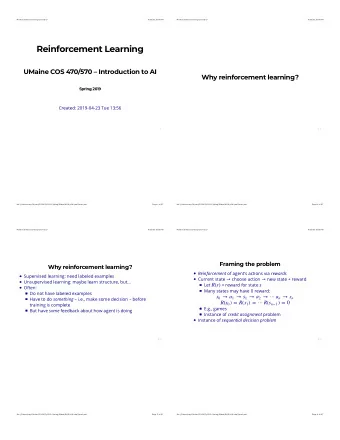
1 Reinforcement Learning • Framework Reinforcement Learning • Rewards, Returns Lectures 4 and 5 • Environment Dynamics Gillian Hayes • Components of a Problem 18th January 2007 • Values and Action Values, V and Q • Optimal Policies • Bellman Optimality Equations Gillian Hayes RL Lecture 4/5 18th January 2007 Gillian Hayes RL Lecture 4/5 18th January 2007 2 3 Framework Again Goals and Rewards Goal: maximise total reward received POLICY State/ Immediate reward r at each step. We must maximise expected cumulative reward: VALUE FUNCTION Situation s t Return = Total reward R t = r t +1 + r t +2 + r t +3 + · · · + r τ AGENT Reward r τ = final time step (episodes/trials) But what if τ = ∞ ? t Action Discounted Reward at r t +1 + γr t +2 + γ 2 r t +3 + · · · Where is boundary R t = r t+1 between agent ∞ and environment? ENVIRONMENT � γ k r t + k +1 = st+1 k =0 Task: one instance of an RL problem – one problem set-up 0 ≤ γ < 1 discount factor → discounted reward finite if reward sequence { r k } Learning: how should agent change policy? bounded Overall goal: maximise amount of reward received over time γ = 0 : myopic γ → 1 : agent far-sighted. Future rewards count for more Gillian Hayes RL Lecture 4/5 18th January 2007 Gillian Hayes RL Lecture 4/5 18th January 2007

4 Dynamics of Environment 5 If action a chosen in state s and subsequent state reached is s ′ what’s the Dynamics of Environment expected reward? Choose action a in situation s : what is the probability of ending up in state s ′ ? Transition probability R a ss ′ = E { r t +1 | s t = s, a t = a, s t +1 = s ′ } ss ′ = Pr { s t +1 = s ′ | s t = s, a t = a } P a If we know P and R then have complete information about environment – may need to learn them BACKUP DIAGRAM s a STOCHASTIC r s’ Gillian Hayes RL Lecture 4/5 18th January 2007 Gillian Hayes RL Lecture 4/5 18th January 2007 6 7 R a ss ′ and ρ ( s, a ) Sutton and Barto’s Recycling Robot 1 Reward functions • At each step, robot has choice of three actions: R a expected next reward given current state s and action a and next state s ′ – go out and search for a can ss ′ ρ ( s, a ) expected next reward given current state s and action a – wait till a human brings it a can – go to charging station to recharge � P a ss ′ R a ρ ( s, a ) = • Searching is better (higher reward), but runs down battery. Running out of ss ′ battery power is very bad and robot needs to be rescued s ′ • Decision based on current state – is energy high or low Sometimes you will see ρ ( s, a ) in the literature, especially that prior to 1998 when • Reward is no. cans (expected to be) collected, negative reward for needing S+B was published. rescue Sometimes you’ll also see ρ ( s ) . This is the reward for being in state s and is equivalent to a “bag of treasure” sitting on a grid-world square (e.g. computer This slide and the next based on an earlier version of Sutton and Barto’s own slides from a games – weapons, health). previous Sutton web resource. Gillian Hayes RL Lecture 4/5 18th January 2007 Gillian Hayes RL Lecture 4/5 18th January 2007

8 9 Sutton and Barto’s Recycling Robot 2 Values V S= { high, low } A(high) = { search, wait } A(low) = { search, wait, recharge } Policy π maps situations s ∈ S to (probability distribution over) actions a ∈ A ( s ) R search expected no. cans when searching R wait expected no. cans when waiting V-Value of s under policy π is V π ( s ) = expected return starting in s and R search > R wait following policy π ∞ search β β ,−3 ,R 1− � V π ( s ) = E π { R t | s t = s } = E π { γ k r t + k +1 | s t = s } wait 1,R wait k =0 search recharge 1,0 BACKUP DIAGRAM FOR V(s) high low s π (s,a) Convention: a open circle = state Pa wait search r filled circle = action ss’ α ,R search wait search α 1,R 1− ,R s’ Gillian Hayes RL Lecture 4/5 18th January 2007 Gillian Hayes RL Lecture 4/5 18th January 2007 10 11 Recursive Relationship for V Action Values Q Q-Action Value of taking action a in state s under policy π is Q π ( s, a ) = V π ( s ) = E π { R t | s t = s } expected return starting in s , taking a and then following policy π ∞ � γ k r t + k +1 | s t = s } = E π { k =0 ∞ � γ k r t + k +2 | s t = s } = E π { r t +1 + γ Q π ( s, a ) = E π { R t | s t = s, a t = a } k =0 ∞ ∞ � γ k r t + k +1 | s t = s, a t = a } = E π { � � P a ss ′ [ R a � γ k r t + k +2 | s t +1 = s ′ } ] = π ( s, a, ) ss ′ + γE π { k =0 a s ′ k =0 � � P a ss ′ [ R a ss ′ + γV π ( s ′ )] = π ( s, a, ) What is the backup diagram? a s ′ This is the BELLMAN EQUATION. How does it relate to backup diagram? Gillian Hayes RL Lecture 4/5 18th January 2007 Gillian Hayes RL Lecture 4/5 18th January 2007

12 13 Recursive Relationship for Q Grid World Example Check the V’s comply with Bellman Equation From Sutton and Barto P. 71, Fig. 3.5 � � Q π ( s, a ) = P a ss ′ [ R a ss ′ + γ π ( s ′ , a ′ ) Q ( s ′ , a ′ )] A B 3.3 8.8 4.4 5.3 1.5 s ′ a ′ +5 1.5 3.0 2.3 1.9 0.5 Relate to backup diagram B’ +10 0.1 0.7 0.7 0.4 -0.4 -1.0 -0.4 -0.4 -0.6 -1.2 A’ -1.9 -1.3 -1.2 -1.4 -2.0 Gillian Hayes RL Lecture 4/5 18th January 2007 Gillian Hayes RL Lecture 4/5 18th January 2007 14 15 Relating Q and V Relating V and Q ∞ ∞ � Q π ( s, a ) γ k r t + k +1 | s t = s, a t = a } = E π { � V π ( s ) γ k r t + k +1 | s t = s } = E π { k =0 k =0 ∞ � π ( s, a ) Q π ( s, a ) = � γ k r t + k +2 | s t = s, a t = a } = E π { r t +1 + γ a k =0 ∞ � � P a ss ′ [ R a γ k r t + k +2 | s t +1 = s ′ } ] = ss ′ + γE π { s ′ k =0 � P a ss ′ [ R a = ss ′ + γV π ( s ′ )] s ′ Gillian Hayes RL Lecture 4/5 18th January 2007 Gillian Hayes RL Lecture 4/5 18th January 2007

16 17 Optimal Policies π ∗ Bellman Optimality Equations 1 An optimal policy has the highest/optimal value function V ∗ ( s ) Bellman equations for the optimal values and Q-values It chooses the action in each state which will result in the highest return Q π ∗ ( s, a ) V ∗ ( s ) = max Optimal Q-value Q ∗ ( s, a ) is reward received from executing action a in state s a and following optimal policy π ∗ thereafter = max E π ∗ { R t | s t = s, a t = a } a � γ k r t + k +2 | s t = s, a t = a } = max E π ∗ { r t +1 + γ a k V π ( s ) V ∗ ( s ) = max = max E { r t +1 + γV ∗ ( s t +1 ) | s t = s, a t = a } π a � P a ss ′ [ R a Q π ( s, a ) ss ′ + γV ∗ ( s ′ )] Q ∗ ( s, a ) = max = max π a s ′ Q ∗ ( s, a ) = E { r t +1 + γV ∗ ( s t +1 ) | s t = s, a t = a } Gillian Hayes RL Lecture 4/5 18th January 2007 Gillian Hayes RL Lecture 4/5 18th January 2007 Bellman Optimality Equations 1 18 19 Bellman Optimality Equations 2 ss ′ known, then can solve equations for V ∗ (or If dynamics of environment R a ss ′ , P a Q ∗ ( s, a ) a ′ Q ∗ ( s t +1 , a ′ ) | s t = s, a t = a } = E { r t +1 + γ max Q ∗ ). � P a ss ′ [ R a a ′ Q ∗ ( s ′ , a ′ )] = ss ′ + γ max Given V ∗ , what then is optimal policy? I.e. which action a do you pick in state s ? s ′ The one which maximises expected r t +1 + γV ∗ ( s t +1 ) , i.e. the one which gives Value under optimal policy = expected return for best action from that state. the biggest s ′ (instant reward + discounted future maximum reward) ∗ P a � ss ′ So need to do one-step search Gillian Hayes RL Lecture 4/5 18th January 2007 Gillian Hayes RL Lecture 4/5 18th January 2007

Bellman Optimality Equations 2 20 21 Assumptions for Solving Bellman Optimality There may be more than one action doing this → all OK Equations All GREEDY actions 1. Know dynamics of environment P a ss ′ , R a ss ′ Given Q ∗ , what’s the optimal policy? 2. Sufficient computational resources (time, memory) BUT The one which gives the biggest Q ∗ ( s, a ) , i.e. in state s , you have various Q Example: Backgammon values, one per action. Pick (an) action with largest Q . 1. OK 2. 10 20 states ⇒ 10 20 equations in 10 20 unknowns, nonlinear equations (max) Often use a neural network to approximate value functions, policies and models ⇒ compact representation Optimal policy? Only needs to be optimal in situations we encounter – some very rarely/never encountered. So a policy that is only optimal in those states we encounter may do Gillian Hayes RL Lecture 4/5 18th January 2007 Gillian Hayes RL Lecture 4/5 18th January 2007 22 Components of an RL Problem 23 Components of an RL Problem • value – V or Q Agent, task, environment • policy States, actions, rewards • model Policy π ( s, a ) → probability of doing a in s Value V ( s ) → number – Value of a state sometimes subject to conditions, e.g. learn best policy you can within given time Action value Q ( s, a ) – Value of a state-action pair Learn to maximise total future discounted reward ss ′ → probability of going from s → s ′ if do a Model P a Reward function R a ss ′ from doing a in s and reaching s ′ Return R → sum of future rewards Total future discounted reward r t +1 + γr t +2 + γ 2 r t +3 + · · · = � ∞ k =0 r t + k +1 γ k Learning strategy to learn... (continued) Gillian Hayes RL Lecture 4/5 18th January 2007 Gillian Hayes RL Lecture 4/5 18th January 2007