Reinforcement Learning Stephen D. Scott (Adapted from Tom Mitchells - PDF document

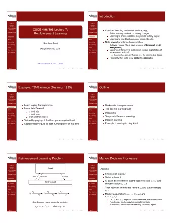
Reinforcement Learning Stephen D. Scott (Adapted from Tom Mitchell’s slides) 1

Outline • Control learning • Control policies that choose optimal actions • Q learning • Convergence • Temporal difference learning 2

Control Learning Consider learning to choose actions, e.g., • Robot learning to dock on battery charger • Learning to choose actions to optimize factory output • Learning to play Backgammon Note several problem characteristics: • Delayed reward (thus have problem of temporal credit assignment) • Opportunity for active exploration (versus exploitation of known good actions) • Possibility that state only partially observable 3

Example: TD-Gammon [Tesauro, 1995] Learn to play Backgammon Immediate Reward: • +100 if win • − 100 if lose • 0 for all other states Trained by playing 1.5 million games against itself 4

Reinforcement Learning Problem Agent State Reward Action Environment a a a 0 1 2 s s s ... 0 1 2 r r r 0 1 2 Goal: Learn to choose actions that maximize 2 γ r + r + ... , where r + 0 < γ <1 γ 0 1 2 5

Markov Decision Processes Assume • Finite set of states S • Set of actions A • At each discrete time agent observes state s t ∈ S and chooses action a t ∈ A • Then receives immediate reward r t , and state changes to s t +1 • Markov assumption: s t +1 = δ ( s t , a t ) and r t = r ( s t , a t ) – I.e., r t and s t +1 depend only on current state and action – Functions δ and r may be nondeterministic – Functions δ and r not necessarily known to agent 6

Agent’s Learning Task Execute actions in environment, observe results, and • learn action policy π : S → A that maximizes r t + γr t +1 + γ 2 r t +2 + . . . � � E from any starting state in S • Here 0 ≤ γ < 1 is the discount factor for future re- wards Note something new: • Target function is π : S → A • But we have no training examples of form � s, a � • Training examples are of form �� s, a � , r � • I.e., not told what best action is, instead told reward for executing action a in state s 7

Value Function First consider deterministic worlds For each possible policy π the agent might adopt, we can define an evaluation function over states ≡ r t + γr t +1 + γ 2 r t +2 + · · · V π ( s ) ∞ γ i r t + i � ≡ i =0 where r t , r t +1 , . . . are generated by following policy π , starting at state s Restated, the task is to learn the optimal policy π ∗ π ∗ ≡ argmax V π ( s ) , ( ∀ s ) π 8

Value Function (cont’d) 0 100 0 G 0 0 0 0 0 100 0 0 0 0 r ( s, a ) (immediate reward) values 0 90 100 G G 90 100 0 81 72 81 81 90 100 81 90 81 90 100 72 81 V ∗ ( s ) values Q ( s, a ) values G 9 One optimal policy

What to Learn We might try to have agent learn the evaluation function V π ∗ (which we write as V ∗ ) It could then do a lookahead search to choose best action from any state s because π ∗ ( s ) = argmax [ r ( s, a ) + γV ∗ ( δ ( s, a ))] a i.e., choose action that maximized immediate reward + discounted reward if optimal strategy followed from then on E.g., V ∗ ( bot. ctr. ) = 0+ γ 100+ γ 2 0+ γ 3 0+ · · · = 90 A problem: • This works well if agent knows δ : S × A → S , and r : S × A → R • But when it doesn’t, it can’t choose actions this way 10

Q Function Define new function very similar to V ∗ : Q ( s, a ) ≡ r ( s, a ) + γV ∗ ( δ ( s, a )) i.e., Q ( s, a ) = total discounted reward if action a taken in state s and optimal choices made from then on If agent learns Q , it can choose optimal action even with- out knowing δ ! π ∗ ( s ) [ r ( s, a ) + γV ∗ ( δ ( s, a ))] = argmax a = argmax Q ( s, a ) a Q is the evaluation function the agent will learn 11

Training Rule to Learn Q Note Q and V ∗ closely related: V ∗ ( s ) = max Q ( s, a ′ ) a ′ Which allows us to write Q recursively as r ( s t , a t ) + γV ∗ ( δ ( s t , a t ))) Q ( s t , a t ) = Q ( s t +1 , a ′ ) = r ( s t , a t ) + γ max a ′ Nice! Let ˆ Q denote learner’s current approximation to Q . Consider training rule Q ( s ′ , a ′ ) ˆ ˆ Q ( s, a ) ← r + γ max a ′ where s ′ is the state resulting from applying action a in state s 12

Q Learning for Deterministic Worlds For each s, a initialize table entry ˆ Q ( s, a ) ← 0 Observe current state s Do forever: • Select an action a (greedily or probabilistically) and execute it • Receive immediate reward r • Observe the new state s ′ • Update the table entry for ˆ Q ( s, a ) as follows: Q ( s ′ , a ′ ) ˆ ˆ Q ( s, a ) ← r + γ max a ′ • s ← s ′ Note that actions not taken and states not seen don’t get explicit updates (might need to generalize) 13

Updating ˆ Q 90 72 100 100 R R 66 66 81 81 a right Initial state: s 1 Next state: s 2 Q ( s 2 , a ′ ) ˆ ˆ Q ( s 1 , a right ) r + γ max ← a ′ = 0 + 0 . 9 max { 66 , 81 , 100 } = 90 Notice if rewards non-negative and ˆ Q ’s initially 0, then ( ∀ s, a, n ) ˆ Q n +1 ( s, a ) ≥ ˆ Q n ( s, a ) and ( ∀ s, a, n ) 0 ≤ ˆ Q n ( s, a ) ≤ Q ( s, a ) (can show via induction on n , using slides 11 and 12) 14

Updating ˆ Q Convergence ˆ Q converges to Q . Consider case of deterministic world where each � s, a � is visited infinitely often. Proof: Define a full interval to be an interval during which each � s, a � is visited. Will show that during each full in- terval the largest error in ˆ Q table is reduced by factor of γ Let ˆ Q n be table after n updates, and ∆ n be the maximum error in ˆ Q n ; i.e., s,a | ˆ ∆ n = max Q n ( s, a ) − Q ( s, a ) | Let s ′ = δ ( s, a ) 15

Updating ˆ Q Convergence (cont’d) For any table entry ˆ Q n ( s, a ) updated on iteration n + 1 , error in the revised estimate ˆ Q n +1 ( s, a ) is | ˆ Q n ( s ′ , a ′ )) ˆ Q n +1 ( s, a ) − Q ( s, a ) | = | ( r + γ max a ′ Q ( s ′ , a ′ )) | − ( r + γ max a ′ Q n ( s ′ , a ′ ) − max ˆ Q ( s ′ , a ′ ) | = γ | max a ′ a ′ | ˆ Q n ( s ′ , a ′ ) − Q ( s ′ , a ′ ) | ( ∗ ) ≤ γ max a ′ Q n ( s ′′ , a ′ ) − Q ( s ′′ , a ′ ) | s ′′ ,a ′ | ˆ ( ∗∗ ) γ max ≤ = γ ∆ n ( ∗ ) works since | max a f 1 ( a ) − max a f 2 ( a ) | ≤ max a | f 1 ( a ) − f 2 ( a ) | ( ∗∗ ) works since max will not decrease Also, ˆ Q 0 ( s, a ) bounded and Q ( s, a ) bounded ∀ s, a ⇒ ∆ 0 bounded Thus after k full intervals, error ≤ γ k ∆ 0 Finally, each � s, a � visited infinitely often ⇒ number of in- tervals infinite, so ∆ n → 0 as n → ∞ 16

Nondeterministic Case What if reward and next state are non-deterministic? We redefine V, Q by taking expected values: r t + γr t +1 + γ 2 r t +2 + · · · � � V π ( s ) ≡ E   ∞ γ i r t + i � = E   i =0 � r ( s, a ) + γV ∗ ( δ ( s, a )) Q ( s, a ) ≡ E � � V ∗ ( δ ( s, a )) = E [ r ( s, a )] + γ E � P ( s ′ | s, a ) V ∗ ( s ′ ) � = E [ r ( s, a )] + γ s ′ P ( s ′ | s, a ) max Q ( s ′ , a ′ ) � = E [ r ( s, a )] + γ a ′ s ′ 17

Nondeterministic Case (cont’d) Q learning generalizes to nondeterministic worlds Alter training rule to Q n − 1 ( s ′ , a ′ )] Q n ( s, a ) ← (1 − α n ) ˆ ˆ ˆ Q n − 1 ( s, a )+ α n [ r + γ max a ′ where 1 α n = 1 + visits n ( s, a ) Can still prove convergence of ˆ Q to Q , with this and other forms of α n [Watkins and Dayan, 1992] 18

Temporal Difference Learning Q learning: reduce error between successive Q ests. Q estimate using one-step time difference: Q (1) ( s t , a t ) ≡ r t + γ max ˆ Q ( s t +1 , a ) a Why not two steps? Q (2) ( s t , a t ) ≡ r t + γr t +1 + γ 2 max ˆ Q ( s t +2 , a ) a Or n ? Q ( n ) ( s t , a t ) ≡ r t + γ r t +1 + · · · + γ ( n − 1) r t + n − 1 + γ n max ˆ Q ( s t + n , a ) a Blend all of these ( 0 ≤ λ ≤ 1 ): � � Q (1) ( s t , a t ) + λQ (2) ( s t , a t ) + λ 2 Q (3) ( s t , a t ) + · · · Q λ ( s t , a t ) (1 − λ ) ≡ � � Q ( s t +1 , a ) + λ Q λ ( s t +1 , a t +1 ) ˆ = r t + γ (1 − λ ) max a TD( λ ) algorithm uses above training rule • Sometimes converges faster than Q learning • converges for learning V ∗ for any 0 ≤ λ ≤ 1 (Dayan, 1992) • Tesauro’s TD-Gammon uses this algorithm 19

Subtleties and Ongoing Research • Replace ˆ Q table with neural net or other generalizer (example is � s, a � , label is ˆ Q ( s, a ) ); convergence proofs break • Handle case where state only partially observable • Design optimal exploration strategies • Extend to continuous action, state • Learn and use ˆ δ : S × A → S • Relationship to dynamic programming (can solve op- timally offline if δ ( s, a ) & r ( s, a ) known) • Reinf. learning in autonomous multi-agent environments (competitive and cooperative) – Now must attribute credit/blame over agents as well as actions – Utilizes game-theoretic techniques, based on agents’ protocols for interacting with environment and each other • More info: survey papers & new textbook 20