REINFORCEMENT LEARNING BANDIT PROBLEMS How does it work? N-armed - PDF document

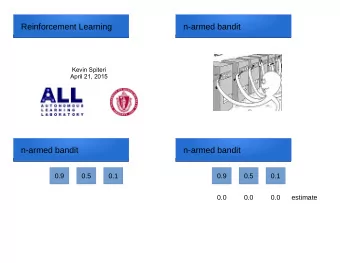
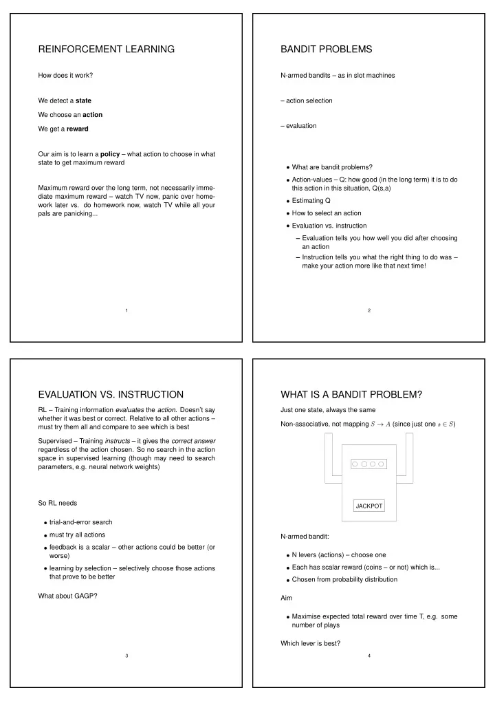
REINFORCEMENT LEARNING BANDIT PROBLEMS How does it work? N-armed bandits – as in slot machines We detect a state – action selection We choose an action – evaluation We get a reward Our aim is to learn a policy – what action to choose in what state to get maximum reward � What are bandit problems? � Action-values – Q: how good (in the long term) it is to do Maximum reward over the long term, not necessarily imme- this action in this situation, Q(s,a) diate maximum reward – watch TV now, panic over home- � Estimating Q work later vs. do homework now, watch TV while all your � How to select an action pals are panicking... � Evaluation vs. instruction – Evaluation tells you how well you did after choosing an action – Instruction tells you what the right thing to do was – make your action more like that next time! 1 2 EVALUATION VS. INSTRUCTION WHAT IS A BANDIT PROBLEM? RL – Training information evaluates the action . Doesn’t say Just one state, always the same whether it was best or correct. Relative to all other actions – ✁ ) ✁✄✂✆☎ Non-associative, not mapping (since just one must try them all and compare to see which is best ✝✟✞ Supervised – Training instructs – it gives the correct answer regardless of the action chosen. So no search in the action space in supervised learning (though may need to search parameters, e.g. neural network weights) So RL needs JACKPOT � trial-and-error search � must try all actions N-armed bandit: � feedback is a scalar – other actions could be better (or � N levers (actions) – choose one worse) � Each has scalar reward (coins – or not) which is... � learning by selection – selectively choose those actions that prove to be better � Chosen from probability distribution What about GAGP? Aim � Maximise expected total reward over time T, e.g. some number of plays Which lever is best? 3 4

✁ ✂ ✝ ✏ ✂ ✌ ✝ ☎ ✁ ✡ ✂ ✪ ✢ ✢ ✍ ✥ ✁ ✁ ✥ ✪ � ✟ ✂ ✝ ✂ ✁ ✏ ✡ ✍ � ✂ ✝ ✟ ✂ ✂ ✦ ACTION VALUE Q ESTIMATING Q ✁✄✂✆☎✞✝✠✟ of action Q value of an action True value ✁☛✡☞☎✞✝✠✟ at play /time Expected/mean reward from that action Estimated value ✝✎✍✑✏ times: If value known exactly, always choose that action Suppose we choose action ✁✄✂ from running mean: ✁☛✡✒☎✞✝✓✟ BUT, only have estimates of Q – build up these estimates Then we can estimate �✕✔✗✖✙✘✠✔✙✚✛✘✠✔✞✜✗✘✣✢ ✘✠✔✛✤ from experience of rewards ✍✧✏ If �✩★✑✪✬✫✮✭✯�✰★ Greedy action(s): have highest estimated Q: EXPLOITA- ✂ ✲✱ ✁✳✡✒☎✞✝✓✟ ✂ ✲✁ ☎✞✝✓✟ As TION ✁ . Sample-average method of calculating Other actions: lower estimated Qs: EXPLORATION ✝✓✟ * in this case means “true value”: Maximise expected reward on 1 play vs. over long time? Uncertainty in our estimates of values of Q EXPLORATION VS. EXPLOITATION TRADEOFF Can’t exploit all the time; must sometimes explore to see if an action that currently looks bad eventually turns out to be good 5 6 ❃ -GREEDY vs. GREEDY ACTION SELECTION � What if reward variance is larger? ✝✴✂ for which Greedy : select the action is highest: � What if reward variance is very small, e.g. zero? ✁☛✡✒☎✞✝✓✂☞✟ ✏✹✁✳✡☞☎ ✝✓✟ �✰✵✷✶✆✸ � What if task is nonstationary? ☎✞✝✓✟ – and * means “best” So �✺✶✼✻✗✽✾✵✄✶✮✸ Exploration and Exploitation again Example : 10-armed bandit Snapshot at time ✌ for actions 1 to 10 ☎✞✝✓✟ 0 0.3 0.1 0.1 0.4 0.05 0 0 0.05 0 ✁☛✡✒☎✞✝ ❀ and ? �✰★✠✿ Maximises immediate reward ❁ -greedy : Select random action ❁ of the time, else select greedy action Sample all actions infinitely many times ✁ ’s converge to ✂ ✲✱ ✁✄✂ So as ❁ over time Can reduce ☎✞✝✓✟ and ✁❂☎ NB: Difference between 7 8

✜ ✆ ✓ ✆ ✓ ✦ ✆ ✔ � ☞ ✘ ✂ ☞ ✦ ✂ ✁ ✥ ✦ ✥ ✁ ✂ ✢ ✘ ✛ � ✘ ★ ✔ ✧ ✍ � ✦ � ✧ ✁ ✡ ✜ ✦ � ✫ ✔ ✡ ✘ ✦ ✁ � ✢ SOFTMAX ACTION SELECTION UPDATE EQUATIONS ✁❂☎✞✝✠✟ Estimate from running mean: if ✔✛✖✙✘✠✔✙✚✛✘✠✔✙✜✛✘✣✢ ✘✠✔✛✤ ✏ times ✝✎✍ ❁ -greedy: if worst action is very bad, will still be chosen with we’ve tried action same probability as second-best – we may not want this. So: Incremental calculation: Vary selection probability as a function of estimated good- (1) ✍ ✙✘✚✔ ☛✌☞ ✴✫ ness ☞✠✤ ✦ ✦✥ (2) ✍ ✙✘✚✔✣✢ ✝ at time Choose ✌ with probability ☎✙✁✳✡✒☎✞✝✓✟ ☎✄✝✆ ✴✟ General form will be met often: ✸ ✂✁ ☎✙✁ ☎ ✏✎ ✆✟ ✑✄✒✆ ✣✟ ✞✠✟ ☛✌☞ ✸ ✍✁ ✆ is temperature (from physics) NewEstimate = OldEstimate + StepSize [ Target - OldEsti- Gibbs/Boltzmann distribution, mate ] ✟ initially very low? ✁❂☎ ✝✴✂ Drawback of softmax? If ✍ in incremental equation: ✔✖✄ Step size depends on Effect of But is often kept constant, e.g. �✩★✑✿ ✂ ✲✱ ✂ ✕✔✖✄✒✗ As , probability (gives more weight to recent rewards – why might this be As ★ , probability greedy useful?) 9 10 EFFECT OF INITIAL VALUES OF Q APPLICATION We arbitrarily set the initial values of Q to be zero. Drug trials. You have a limited number of trials, several drugs, and need to choose the best of them. Bandit arm Biassed by initial estimate of Q drug Can use this to include domain knowledge Define a measure of success/failure – the reward Example Set all Q values very high – optimistic Ethical clinical trials – how do we allocate patients to drug treatments? During the trial we may find that some drugs Initial actual rewards are disappointing compared to esti- work better than others. mate, so switch to another action – exploration � Fixed allocation design: allocate ✔✖✄ ✧✍ Temporary effect of the patients to ✍ drugs each of the � Adaptive allocation design: if the patients on one drug POLICY appear to be doing better, switch others to that drug – equivalent to removing one of the arms of the bandit Once we’ve learnt the Q values, our policy is the greedy one: choose the action with the highest Q See: http://www.eecs.umich.edu/ ✩ qstout/AdaptSample.html And: J.Hardwick, R.Oehmke,Q.Stout: A program for sequen- tial allocation of three Bernoulli populations, Computational Statistics and Data Analysis 31, 397–416, 1999. (just scan this one) 11 12