Reinforcement Learning Algorithms A. LAZARIC ( SequeL Team - PowerPoint PPT Presentation
Reinforcement Learning Algorithms A. LAZARIC ( SequeL Team @INRIA-Lille ) ENS Cachan - Master 2 MVA SequeL INRIA Lille MVA-RL Course In This Lecture How do we solve an MDP online? RL Algorithms A. LAZARIC Reinforcement Learning
Reinforcement Learning Algorithms A. LAZARIC ( SequeL Team @INRIA-Lille ) ENS Cachan - Master 2 MVA SequeL – INRIA Lille MVA-RL Course
In This Lecture ◮ How do we solve an MDP online? ⇒ RL Algorithms A. LAZARIC – Reinforcement Learning Algorithms Oct 15th, 2013 - 2/76
In This Lecture ◮ Dynamic programming algorithms require an explicit definition of ◮ transition probabilities p ( ·| x , a ) ◮ reward function r ( x , a ) ◮ This knowledge is often unavailable (i.e., wind intensity, human-computer-interaction). ◮ Can we relax this assumption? A. LAZARIC – Reinforcement Learning Algorithms Oct 15th, 2013 - 3/76
In This Lecture ◮ Learning with generative model. A black-box simulator f of the environment is available. Given ( x , a ) , f ( x , a ) = { y , r } with y ∼ p ( ·| x , a ) , r = r ( x , a ) . ◮ Episodic learning. Multiple trajectories can be repeatedly generated from the same state x and terminating when a reset condition is achieved: ( x i 0 = x , x i 1 , . . . , x i T i ) n i = 1 . ◮ Online learning. At each time t the agent is at state x t , it takes action a t , it observes a transition to state x t + 1 , and it receives a reward r t . We assume that x t + 1 ∼ p ( ·| x t , a t ) and r t = r ( x t , a t ) (i.e., MDP assumption). A. LAZARIC – Reinforcement Learning Algorithms Oct 15th, 2013 - 4/76
Mathematical Tools Outline Mathematical Tools The Monte-Carlo Algorithm The TD(1) Algorithm The TD(0) Algorithm The TD( λ ) Algorithm The Q -learning Algorithm A. LAZARIC – Reinforcement Learning Algorithms Oct 15th, 2013 - 5/76
Mathematical Tools Concentration Inequalities Let X be a random variable and { X n } n ∈ N a sequence of r.v. a . s . ◮ { X n } converges to X almost surely , X n − → X , if P ( lim n →∞ X n = X ) = 1 , P ◮ { X n } converges to X in probability , X n − → X , if for any ǫ > 0, n →∞ P [ | X n − X | > ǫ ] = 0 , lim D ◮ { X n } converges to X in law (or in distribution), X n − → X , if for any bounded continuous function f n →∞ E [ f ( X n )] = E [ f ( X )] . lim a . s . P D Remark: X n − → X = ⇒ X n − → X = ⇒ X n − → X . A. LAZARIC – Reinforcement Learning Algorithms Oct 15th, 2013 - 6/76
Mathematical Tools Concentration Inequalities Proposition (Markov Inequality) Let X be a positive random variable. Then for any a > 0, P ( X ≥ a ) ≤ E X a . Proof. P ( X ≥ a ) = E [ I { X ≥ a } ] = E [ I { X / a ≥ 1 } ] ≤ E [ X / a ] � A. LAZARIC – Reinforcement Learning Algorithms Oct 15th, 2013 - 7/76
Mathematical Tools Concentration Inequalities Proposition (Hoeffding Inequality) Let X be a centered random variable bounded in [ a , b ] . Then for any s ∈ R , E [ e sX ] ≤ e s 2 ( b − a ) 2 / 8 . A. LAZARIC – Reinforcement Learning Algorithms Oct 15th, 2013 - 8/76
Mathematical Tools Concentration Inequalities Proof. From convexity of the exponential function, for any a ≤ x ≤ b , e sx ≤ x − a b − ae sb + b − x b − a e sa . Let p = − a / ( b − a ) then (recall that E [ X ] = 0) b a b − ae sa − E [ e sx ] b − ae sb ≤ ( 1 − p + pe s ( b − a ) ) e − ps ( b − a ) = e φ ( u ) = with u = s ( b − a ) and φ ( u ) = − pu + log ( 1 − p + pe u ) whose derivative is p φ ′ ( u ) = − p + p + ( 1 − p ) e − u , p ( 1 − p ) e − u and φ ( 0 ) = φ ′ ( 0 ) = 0 and φ ′′ ( u ) = ( p +( 1 − p ) e − u ) 2 ≤ 1 / 4. Thus from Taylor’s theorem , the exists a θ ∈ [ 0 , u ] such that φ ( θ ) = φ ( 0 ) + θφ ′ ( 0 ) + u 2 2 φ ′′ ( θ ) ≤ u 2 8 = s 2 ( b − a ) 2 . 8 A. LAZARIC – Reinforcement Learning Algorithms Oct 15th, 2013 - 9/76
Mathematical Tools Concentration Inequalities Proposition (Chernoff-Hoeffding Inequality) Let X i ∈ [ a i , b i ] be n independent r.v. with mean µ i = E X i . Then �� �� � � � n � 2 ǫ 2 � � � X i − µ i � ≥ ǫ ≤ 2 exp − � n . P � i = 1 ( b i − a i ) 2 i = 1 A. LAZARIC – Reinforcement Learning Algorithms Oct 15th, 2013 - 10/76
Mathematical Tools Concentration Inequalities Proof. � � n � P ( e s � n i = 1 X i − µ i ≥ e s ǫ ) X i − µ i ≥ ǫ = P i = 1 e − s ǫ E [ e s � n i = 1 X i − µ i ] , ≤ Markov inequality n � e − s ǫ E [ e s ( X i − µ i ) ] , = independent random variables i = 1 n � e s 2 ( b i − a i ) 2 / 8 , e − s ǫ ≤ Hoeffding inequality i = 1 e − s ǫ + s 2 � n i = 1 ( b i − a i ) 2 / 8 = If we choose s = 4 ǫ/ � n i = 1 ( b i − a i ) 2 , the result follows. � � n � Similar arguments hold for P i = 1 X i − µ i ≤ − ǫ . A. LAZARIC – Reinforcement Learning Algorithms Oct 15th, 2013 - 11/76
Mathematical Tools Monte-Carlo Approximation of a Mean Definition Let X be a random variable with mean µ = E [ X ] and variance σ 2 = V [ X ] and x n ∼ X be n i.i.d. realizations of X. The Monte-Carlo approximation of the mean (i.e., the empirical mean) built on n i.i.d. realizations is defined as n � µ n = 1 x i . n i = 1 A. LAZARIC – Reinforcement Learning Algorithms Oct 15th, 2013 - 12/76
Mathematical Tools Monte-Carlo Approximation of a Mean ◮ Unbiased estimator : Then E [ µ n ] = µ (and V [ µ n ] = V [ X ] n ) P ◮ Weak law of large numbers: µ n − → µ . a . s . ◮ Strong law of large numbers : µ n − → µ . ◮ Central limit theorem (CLT) : √ n ( µ n − µ ) D − → N ( 0 , V [ X ]) . ◮ Finite sample guarantee : � � � � � � � n 2 n ǫ 2 � 1 � � X t − E [ X 1 ] � > ǫ ≤ 2 exp − P ���� ( b − a ) 2 n � �� � t = 1 accuracy � �� � confidence deviation A. LAZARIC – Reinforcement Learning Algorithms Oct 15th, 2013 - 13/76
Mathematical Tools Monte-Carlo Approximation of a Mean ◮ Unbiased estimator : Then E [ µ n ] = µ (and V [ µ n ] = V [ X ] n ) P ◮ Weak law of large numbers: µ n − → µ . a . s . ◮ Strong law of large numbers : µ n − → µ . ◮ Central limit theorem (CLT) : √ n ( µ n − µ ) D − → N ( 0 , V [ X ]) . ◮ Finite sample guarantee : �� � � � n � � 1 log 2 /δ � � X t − E [ X 1 ] � > ( b − a ) ≤ δ P n 2 n t = 1 A. LAZARIC – Reinforcement Learning Algorithms Oct 15th, 2013 - 14/76
Mathematical Tools Monte-Carlo Approximation of a Mean ◮ Unbiased estimator : Then E [ µ n ] = µ (and V [ µ n ] = V [ X ] n ) P ◮ Weak law of large numbers: µ n − → µ . a . s . ◮ Strong law of large numbers : µ n − → µ . ◮ Central limit theorem (CLT) : √ n ( µ n − µ ) D − → N ( 0 , V [ X ]) . ◮ Finite sample guarantee : �� � � n � � 1 � � X t − E [ X 1 ] � > ǫ ≤ δ P n t = 1 if n ≥ ( b − a ) 2 log 2 /δ . 2 ǫ 2 A. LAZARIC – Reinforcement Learning Algorithms Oct 15th, 2013 - 15/76
Mathematical Tools Exercise Simulate n Bernoulli of probability p and verify the correctness and the accuracy of the C-H bounds. A. LAZARIC – Reinforcement Learning Algorithms Oct 15th, 2013 - 16/76
Mathematical Tools Stochastic Approximation of a Mean Definition Let X a random variable bounded in [ 0 , 1 ] with mean µ = E [ X ] and x n ∼ X be n i.i.d. realizations of X. The stochastic approximation of the mean is, µ n = ( 1 − η n ) µ n − 1 + η n x n with µ 1 = x 1 and where ( η n ) is a sequence of learning steps. Remark: When η n = 1 n this is the recursive definition of empirical mean. A. LAZARIC – Reinforcement Learning Algorithms Oct 15th, 2013 - 17/76
Mathematical Tools Stochastic Approximation of a Mean Proposition (Borel-Cantelli) Let ( E n ) n ≥ 1 be a sequence of events such that � n ≥ 1 P ( E n ) < ∞ , then the probability of the intersection of an infinite subset is 0. More formally, � � � ∞ � ∞ � � lim sup n →∞ E n = P E k = 0 . P n = 1 k = n A. LAZARIC – Reinforcement Learning Algorithms Oct 15th, 2013 - 18/76
Mathematical Tools Stochastic Approximation of a Mean Proposition If for any n , η n ≥ 0 and are such that � � η 2 η n = ∞ ; n < ∞ , n ≥ 0 n ≥ 0 then a . s . µ n − → µ, and we say that µ n is a consistent estimator. A. LAZARIC – Reinforcement Learning Algorithms Oct 15th, 2013 - 19/76
Mathematical Tools Stochastic Approximation of a Mean Proof. We focus on the case η n = n − α . In order to satisfy the two conditions we need 1 / 2 < α ≤ 1. In fact, for instance � n 2 = π 2 1 α = 2 ⇒ 6 < ∞ (see the Basel problem) n ≥ 0 � 1 � 2 � � 1 α = 1 / 2 ⇒ √ n n = ∞ = (harmonic series) . n ≥ 0 n ≥ 0 A. LAZARIC – Reinforcement Learning Algorithms Oct 15th, 2013 - 20/76
Mathematical Tools Stochastic Approximation of a Mean Proof (cont’d). Case α = 1 Let ( ǫ k ) k a sequence such that ǫ k → 0, almost sure convergence corresponds to � � � � � ≤ ǫ k ) = 1 . � µ n − µ n →∞ µ n = µ lim = P ( ∀ k , ∃ n k , ∀ n ≥ n k , P From Chernoff-Hoeffding inequality for any fixed n �� � � � ≥ ǫ ≤ 2 e − 2 n ǫ 2 . � µ n − µ (1) P � � � ≥ ǫ } . From C-H � µ n − µ Let { E n } be a sequence of events E n = { � P ( E n ) < ∞ , n ≥ 1 and from Borel-Cantelli lemma we obtain that with probability 1 there � � � µ n − µ � ≥ ǫ . exist only a finite number of n values such that A. LAZARIC – Reinforcement Learning Algorithms Oct 15th, 2013 - 21/76
Recommend
More recommend
Explore More Topics
Stay informed with curated content and fresh updates.
